Understanding Interactions in Linear Models

When we consider the set of predictors for a linear model, we’re often imagining interactions as well, even if we don’t realize it. A model with no interaction terms between predictors actually takes a pretty strong stance — that all of the effects are totally independent — which you may not be comfortable with. This post will walk you through how adding an interaction term between a continuous and a categorical predictor changes your model, both statistically and in terms of your real-world interpretation of results.

For example, consider a model where we predict severity of asthma symptoms (outcome) from a genetic predisposition (yes/no) and a rating of environmental hazards (I am not a clinician, so please forgive my ridiculously vague variables). Here are the first five cases from the made-up data:

# this is the code to generate the made-up data
n <- 100
mutation_present <- factor(sample(c("Y", "N"), size = n, replace = TRUE))
hazards <- runif(n = n, min = 1, max = 10)
asthma_sx <- rnorm(n = n, mean = 0, sd = 5) + 50 + 
  ifelse(mutation_present == "N", .5*(hazards - mean(hazards)), 3 + 3*(hazards - mean(hazards)))

asthma <- data.frame(asthma_sx, mutation_present, hazards)

asthma\_sx	mutation\_present	hazards
51.01146	Y	3.948626
41.62890	Y	1.806636
43.28245	N	2.142964
43.62257	N	7.350567
48.59636	N	8.387239

The main effects model

Let’s say we hypothesize that both the genetic predisposition and the degree of environmental hazards present will predict severity of asthma symptoms. We can articulate that in a linear model with asthma_sx as the outcome, and mutation_present and hazards as predictors.

Before we run the model, though, we need to do a little preparation with the data. In general, it’s wise to center any continuous predictors before entering them in your model. We have one continuous predictor here, hazards, so we’ll center it now:

# center hazards by subtracting the mean from each observation
asthma$hazards <- asthma$hazards - mean(asthma$hazards, na.rm = TRUE)

It’s also very important to check how R is interpreting your variables, to make sure it’s understanding categorical variables as factors. If R thinks a variable is numeric when it’s supposed to be categorical, your results will be nonsense (except in the special case of binary categorical variables coded as 0 or 1). We can check to make sure R is seeing mutation_present as a factor with the str command:

str(asthma)

'data.frame':   100 obs. of  3 variables:
 $ asthma_sx       : num  51 41.6 43.3 43.6 48.6 ...
 $ mutation_present: Factor w/ 2 levels "N","Y": 2 2 1 1 1 2 2 2 2 2 ...
 $ hazards         : num  -1.15 -3.3 -2.96 2.25 3.28 ...

Looks good. We can run the model now. I’ve done it here in R code, but you could run the equivalent model in any statistical software.

# a linear model with only main effects for hazard and mutation_present
model_mains <- lm(asthma_sx ~ hazards + mutation_present, data = asthma)

# show a model summary, giving the estimates of the coefficients
summary(model_mains)


Call:
lm(formula = asthma_sx ~ hazards + mutation_present, data = asthma)

Residuals:
     Min       1Q   Median       3Q      Max 
-10.9476  -4.4159   0.0298   4.6779  11.4855 

Coefficients:
                  Estimate Std. Error t value Pr(>|t|)    
(Intercept)        49.8253     0.7920  62.911  < 2e-16 ***
hazards             1.6649     0.2194   7.589 1.98e-11 ***
mutation_presentY   3.6452     1.1470   3.178  0.00199 ** 
---
Signif. codes:  0 '***' 0.001 '**' 0.01 '*' 0.05 '.' 0.1 ' ' 1

Residual standard error: 5.693 on 97 degrees of freedom
Multiple R-squared:  0.4332,    Adjusted R-squared:  0.4215 
F-statistic: 37.07 on 2 and 97 DF,  p-value: 1.101e-12

What may not be immediately apparent is that by only including each predictor as a independent variable, we are explicitly saying that the interaction between these two terms is 0. In other words, we are stating that the effect of environmental hazards on asthma symptoms is the same for patients with and without the genetic predisposition, and that the effect of having the genetic predisposition on asthma symptoms is the same regardless of any environmental hazards the patient may be exposed to.

Hopefully that’s ringing alarm bells for you. A much more natural hypothesis in this situation is that both the genetic predisposition and environmental hazards matter for asthma symptoms, but that also the effect of each depends in part on the other.

For example, the impact of environmental hazards may be relatively small in patients with no genetic predisposition, but exposure to hazards may be a much stronger predictor of symptom severity in patients who do have the relevant genetic mutation. Similarly, while having a genetic predisposition may be associated with more severe asthma symptoms in general, maybe that difference is pretty minor where there are few environmental hazards and much stronger when hazards are more prevalent. In either case, what we’re talking about here is a statistical interaction between hazards and mutation_present (note that although we may think and talk about interactions as either “the effect of A depends on B” or “the effect of B depends on A”, statistically those two things are the same, and both are represented by the single A:B interaction term).

Without the interaction, we’re modeling just the main effects of hazards and mutation_present. In a linear regression model, this could be represented with the following equation (if mathematical equations don’t help you, feel free to gloss over this bit and join us again at the plot):

$asthma\_sx_i=\beta_0+\beta_1hazards_i+\beta_2mutation\_present_i+e_i$

Where the severity of asthma symptoms for patient $i$ equals some constant $\beta_0$ (also called the intercept) plus $\beta_1$ times patient $i$ ’s hazard rating plus $\beta_2$ times 1 if patient $i$ has the mutation or 0 if they don’t, plus some random error $e$ . To see how this actually generates lines of best fit, we can fill in parts of the equation and see how it changes. For example, if a patient does not have the genetic predisposition for asthma (mutation_present=0), then their line would be $\beta_0 + \beta_1*hazard + \beta_2*0$ , which simplifies to just $\beta_0 + \beta_1*hazard$ . If a patient does have the genetic predisposition (mutatation_present=1), then it would be $\beta_0 + \beta_1*hazard + \beta_2*1$ , or combining like terms $(\beta_0 + \beta_2) + \beta_1*hazard$ . In other words, the intercept changes depending on whether or not the patient has the mutation, but you can see the slope for hazard is still just $\beta_1$ in either case.

We can estimate the values for each of the $\beta$ parameters by running the linear regression model above. The results of that model tell us that the estimate for $\beta_0$ is r round(model_mains$coef[1], 2), for $\beta_1$ it’s r round(model_mains$coef[2], 2) and for $\beta_2$ it’s r round(model_mains$coef[3], 2). We can see the lines of best fit for each group clearly by plotting the regression lines for those with the mutation and not separately (I’m using the ggplot2 package for plotting here, see this post for an overview if you want to understand the following R code better):

library(ggplot2)

ggplot(asthma, aes(y=asthma_sx, x=hazards, color=mutation_present)) + 
  # make a scatter plot
  geom_point() + 
  # overlay best fit lines from the model object saved above
  geom_line(aes(y=predict(model_mains))) + 
  # change theme to give it a white background and cleaner appearance
  theme_bw() + 
  # manually set the labels
  labs(y="Asthma Symptoms", x = "Environmental Hazards Rating", color = "Mutation\nPresent",
       title="Model with main effects only") + 
  # use a separate pane for each value of mutation_present (N or Y)
  facet_wrap(~mutation_present)

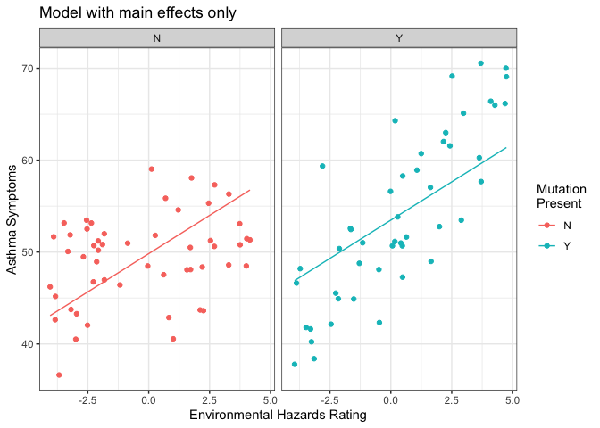
This plot shows our patients with and without the genetic mutation separately, and the line overlaid on each is the line of best fit predicted from the model we just ran. There are two main things to notice here:

The slope of the line (i.e. the strength of the effect of environmental hazards on severity of asthma symptoms) is exactly the same in both plots — those two lines are parallel.
Neither line is a super good fit for the data it describes. Imagine tilting each line a little bit to make it run more directly through its cloud of points.

How the model changes with an interaction term included

If we add an interaction term to the model, we effectively allow the model to fit a different slope for hazards in the two mutation groups. You can see how that works by taking a look at how the the model equation changes with an interaction term included:

$asthma\_sx_i=\beta_0+\beta_1hazards_i+\beta_2mutation\_present_i+\beta_3hazards*mutation\_present+e_i$

Now, for a patient without the genetic predisposition for asthma (mutation_present=0), their equation would simplify to $\beta_0 + \beta_1*hazards + \beta_2*0 + \beta3*hazards*0$ , and the 0 terms drop out leaving us with $\beta_0 + \beta_1*hazards$ . For patients with the genetic predisposition (mutation_present=1), their equation would simplify to $\beta_0 + \beta_1*hazards + \beta_2*1 + \beta3*hazards*1$ , and if we combine like terms we get $(\beta_0 + \beta_2) +(\beta_1+\beta3)*hazards$ . Both the intercept and the slope change depending on whether patients have the mutation. Here is the R code[^interaction-only] to run the model including an interaction term.

# a linear model including both main effects and their interaction
model_int <- lm(asthma_sx ~ hazards * mutation_present, data = asthma)

# show the estimates of model cofficients
summary(model_int)


Call:
lm(formula = asthma_sx ~ hazards * mutation_present, data = asthma)

Residuals:
     Min       1Q   Median       3Q      Max 
-10.8270  -3.3018  -0.3596   3.4391  14.3996 

Coefficients:
                          Estimate Std. Error t value Pr(>|t|)    
(Intercept)                49.5104     0.6716  73.723  < 2e-16 ***
hazards                     0.5602     0.2553   2.194 0.030626 *  
mutation_presentY           3.5786     0.9700   3.689 0.000373 ***
hazards:mutation_presentY   2.3401     0.3716   6.298 9.08e-09 ***
---
Signif. codes:  0 '***' 0.001 '**' 0.01 '*' 0.05 '.' 0.1 ' ' 1

Residual standard error: 4.814 on 96 degrees of freedom
Multiple R-squared:  0.5989,    Adjusted R-squared:  0.5864 
F-statistic: 47.78 on 3 and 96 DF,  p-value: < 2.2e-16

And here is a plot showing the data, separated by whether patients have the genetic mutation or not, with lines of best fit from the model overlaid.

ggplot(asthma, aes(y=asthma_sx, x=hazards, color=mutation_present)) + 
  # make a scatter plot
  geom_point() + 
  # overlay best fit lines from the model object saved above
  geom_line(aes(y=predict(model_int))) + 
  # change theme to give it a white background and cleaner appearance
  theme_bw() + 
  # manually set the labels
  labs(y="Asthma Symptoms", x = "Environmental Hazards Rating", color = "Mutation\nPresent",
       title="Model including interaction") + 
  # use a separate pane for each value of mutation_present (0 or 1)
  facet_wrap(~mutation_present)

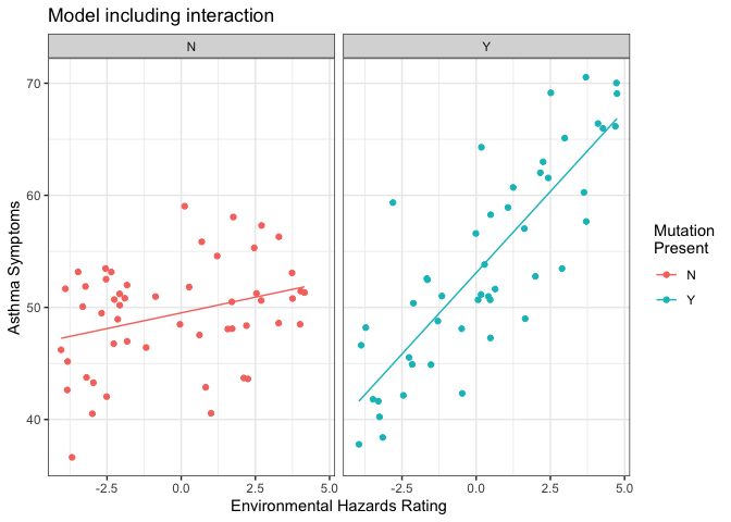
As you can see, the regression lines do a much better job of describing the data here, when we allow the model to fit a separate slope and intercept for each group. Statistically, this is reflected in the tests of the model coefficients (we get a significant t-test for the interaction term in the model), and in the improvement in overall model fit when we go from the main effects only model to the one including the interaction term:

# test the change in model fit from the main effects model to the interaction model
anova(model_mains, model_int)

Analysis of Variance Table

Model 1: asthma_sx ~ hazards + mutation_present
Model 2: asthma_sx ~ hazards * mutation_present
  Res.Df    RSS Df Sum of Sq     F    Pr(>F)    
1     97 3144.2                                 
2     96 2225.0  1     919.2 39.66 9.076e-09 ***
---
Signif. codes:  0 '***' 0.001 '**' 0.01 '*' 0.05 '.' 0.1 ' ' 1

The take-away: Whether or not you include interaction terms, think about the assumptions your model makes

Unfortunately, the solution isn’t as simple as “always include interaction terms” — sometimes the interaction wouldn’t make sense theoetically, and often including interaction terms (especially several interactions at once, or more complex terms like three-way interactions) makes your model more difficult to interpret. There is also a serious risk of overfitting the data: making a model so closely tuned to your specific dataset that it loses its value for prediction to new data. The model discussed here is relatively simple, with only two predictive variables, but if you have a more complex model and you allow interactions among all of your predictors, you can easily end up overfitting.

The thing to keep in mind is that whatever statistical model you use, it is stating a hypothesis about the variables you include, but also making the assumption that the coefficient is 0 for all of the variables you omit. For many omitted variables, including omited interaction terms, you will feel fine about making that assumption (even if it’s not strictly accurate) — but it’s important to remember that you’re making it. In the words of famous statistician George Box: “Remember that all models are wrong; the practical question is how wrong do they have to be to not be useful.”

[1] What if you put in only the interaction with no main effects? You may notice I don’t separately write out each main effect here, like asthma_sx ~ hazards + mutation_present + hazards:mutation_present. That’s because R assumes you will always want both main effects when you include an interaction, so A*B is a shorthand that includes both main effects and the interaction: A + B + A:B. Except in pretty unusual circumstances, it’s not a good idea to try to run a model with an interaction but without one or both main effects since it can substantially change the interpretation of your coefficients. Read more here about what happens when you include an interaction term without its main effects.

Like this article? Click "Like" to let us know.

Tags

Understanding Interactions in Linear Models

The main effects model

How the model changes with an interaction term included

The take-away: Whether or not you include interaction terms, think about the assumptions your model makes