Ordinary Linear Regression in R

Linear regression in R

Linear regression is the process of creating a model of how one or more explanatory or independent variables change the value of an outcome or dependent variable, when the outcome variable is not dichotomous (2-valued). When the outcome is dichotomous (e.g. “Male” / “Female”, “Survived” / “Died”, etc.), a logistic regression is more appropriate.

When we first learn linear regression we typically learn ordinary regression (or “ordinary least squares”), where we assert that our outcome variable must vary according to a linear combination of explanatory variables. We end up, in ordinary linear regression, with a straight line through our data. This line has a formula that’s very reminiscent of the line equations we learned in Algebra I as teenagers:

Where $\alpha$ (sometimes $\beta_0$) is the y-intercept, and the other $\beta$ are the coefficients corresponding to each predictor variable. You may also see this formula with an “error term” $\epsilon$ added, which is the “noise” our model can’t account for. This is pretty similar to $y=mx+b$, right?

There’s another type of linear regression with greater flexibility, called GLM, or generalized linear modeling, which we’ll address in a future article. The benefits of GLM include getting a prediction curve that isn’t necessarily a straight line and prediction that makes sense for non-normally distributed outcomes. GLM is very powerful, and deserves its own treatment. For now, we’ll stick with ordinary linear regression, for one predictor variable (simple linear regression) and for multiple predictor variables (multiple linear regression). We’ll address this in two main sections: Simple Linear Regression and Multiple Regression.

Simple Linear Regression

Let’s take simple linear regression first. What we’re trying to do is reduce the sum of squares of all our residuals (i.e. create a line that passes through our data points as closely as possible). At the end of the day, this is an optimization project that calls for calculus and uses the correlation coefficient $r$. To find out more about the math that calculates the best line (“best” here means with the lowest sum of squared errors), check out the Khan Academy treatment of the subject. We’ll end up with a slope ($r\cdot\frac{s_y}{s_x}$, where s = sample standard deviation) and a point $(\bar{x},\bar{y}$), which, from Algebra I, we know we can put into the formula for a line (the point-slope formula). Usually, you won’t bother calculating all of this yourself, but it’s handy to recognize the relationship between some basic descriptive statistics and how your model is formed.

In R, it’s fairly simple to create a linear model using lm and formula notation, where we model an output ~ input, where we can interpret ~ as “as a function of” . Let’s take the mtcars dataset, which ships with base R, and do a bit of linear modeling:

data(mtcars)
my_model <- lm(mpg ~ wt, mtcars)
my_model
summary(my_model)

You should get the following output:

> my_model

Call:
lm(formula = mpg ~ wt, data = mtcars)

Coefficients:
(Intercept)           wt  
     37.285       -5.344  

> summary(my_model)

Call:
lm(formula = mpg ~ wt, data = mtcars)

Residuals:
    Min      1Q  Median      3Q     Max 
-4.5432 -2.3647 -0.1252  1.4096  6.8727 

Coefficients:
            Estimate Std. Error t value Pr(>|t|)    
(Intercept)  37.2851     1.8776  19.858  < 2e-16 ***
wt           -5.3445     0.5591  -9.559 1.29e-10 ***
---
Signif. codes:  0 ‘***’ 0.001 ‘**’ 0.01 ‘*’ 0.05 ‘.’ 0.1 ‘ ’ 1

Residual standard error: 3.046 on 30 degrees of freedom
Multiple R-squared:  0.7528,	Adjusted R-squared:  0.7446 
F-statistic: 91.38 on 1 and 30 DF,  p-value: 1.294e-10

We can see that summary() gives us a bit more detail than just the slope and intercept: it gives us the statistical significance of these values, as well as our R-squared value, which is a measure of how much of the behavior of the outcome variable is explained by our model. In our case, we have an R-squared value of 0.7528, or, if we’re adjusting for the number of variables used (a good idea, especially since we’ll start doing multiple regression), 0.7446. So we have between 74% and 75% of the variation in mpg (miles per gallon fuel economy) explained by just wt (weight in thousands of pounds). Not too bad! Additionally we see that both our intercept and the coefficient for wt are highly statistically significant. Let’s plot both the points and our model (a straight line with a y-intercept of 37.2851 and a slope of -5.3445):

library(ggplot2)
ggplot(mtcars, aes(wt, mpg)) +
  geom_point() +
  geom_abline(intercept = 37.2851, slope = -5.3445, color = "red")

Or, you could also access the slope and intercept directly, like this:

library(ggplot2)
ggplot(mtcars, aes(wt, mpg)) +
  geom_point() +
  geom_abline(intercept = my_model$coefficients[1], 
              slope = my_model$coefficients[2], 
              color = "red")

Either should give you something like the following:

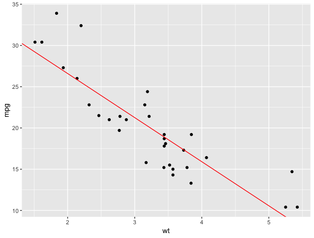
That’s a fairly good model. Visually, we see that it cuts through the points without any clear pattern of residuals (the points are scattered randomly above and below the line). Statistically, we see a good R-squared and convincing p-values. I’d feel comfortable saying this model does a good job of predicting MPG, given automotive weight.

Multiple Linear Regression

Since mtcars has a lot of variables, let’s not stop at just one explanatory variable.

Main Effects

Let’s say we want to predict mpg as a function of both weight and transmission type. Since am is really a factor variable (0 = automatic, 1 = manual), we’ll put in as.factor(). This may seem like overkill, as lm will figure out that this is a factor on its own, but it’s always a helpful reminder both for R and for us that we’re dealing with a factor variable.

This is a model that looks at main effects only (weight’s influence alone, considering nothing else, and transmission type alone, considering nothing else).

First of all, does it matter what order we put our explanatory variables? Let’s check, and try both orders. Note that we separate effects with a plus sign (+).

my_multi_model_1 <- lm(mpg ~ wt + as.factor(am), mtcars)
my_multi_model_2 <- lm(mpg ~ as.factor(am) + wt, mtcars)
summary(my_multi_model_1)
summary(my_multi_model_2)

You should get the following output:

> summary(my_multi_model_1)

Call:
lm(formula = mpg ~ wt + as.factor(am), data = mtcars)

Residuals:
    Min      1Q  Median      3Q     Max 
-4.5295 -2.3619 -0.1317  1.4025  6.8782 

Coefficients:
               Estimate Std. Error t value Pr(>|t|)    
(Intercept)    37.32155    3.05464  12.218 5.84e-13 ***
wt             -5.35281    0.78824  -6.791 1.87e-07 ***
as.factor(am)1 -0.02362    1.54565  -0.015    0.988    
---
Signif. codes:  0 ‘***’ 0.001 ‘**’ 0.01 ‘*’ 0.05 ‘.’ 0.1 ‘ ’ 1

Residual standard error: 3.098 on 29 degrees of freedom
Multiple R-squared:  0.7528,	Adjusted R-squared:  0.7358 
F-statistic: 44.17 on 2 and 29 DF,  p-value: 1.579e-09

> summary(my_multi_model_2)

Call:
lm(formula = mpg ~ as.factor(am) + wt, data = mtcars)

Residuals:
    Min      1Q  Median      3Q     Max 
-4.5295 -2.3619 -0.1317  1.4025  6.8782 

Coefficients:
               Estimate Std. Error t value Pr(>|t|)    
(Intercept)    37.32155    3.05464  12.218 5.84e-13 ***
as.factor(am)1 -0.02362    1.54565  -0.015    0.988    
wt             -5.35281    0.78824  -6.791 1.87e-07 ***
---
Signif. codes:  0 ‘***’ 0.001 ‘**’ 0.01 ‘*’ 0.05 ‘.’ 0.1 ‘ ’ 1

Residual standard error: 3.098 on 29 degrees of freedom
Multiple R-squared:  0.7528,	Adjusted R-squared:  0.7358 
F-statistic: 44.17 on 2 and 29 DF,  p-value: 1.579e-09

There’s no difference in the intercept, coefficients, or statistical metrics. Variable order does not matter in lm.

The three coefficients represent the y-intercept, a tiny amount to subtract if the transmission is a manual (am = 1), and the coefficient for the weight variable. Our formula would be something like:

*(Only if car is manual)

We’d have the same slope, but different y-intercepts (but barely!)

We could plot it like this. Note that the lines are very hard to distinguish as they almost coincide:

ggplot(mtcars, aes(wt, mpg)) +
  geom_point(aes(color=as.factor(am))) +
  scale_color_manual(values=c("red", "blue")) +
  geom_abline(intercept = my_multi_model_1$coefficients[1], 
              slope = my_multi_model_1$coefficients[2], 
              color = "red") +
  geom_abline(intercept = my_multi_model_1$coefficients[1] +
                my_multi_model_1$coefficients[3], 
              slope = my_multi_model_1$coefficients[2], 
              color = "blue")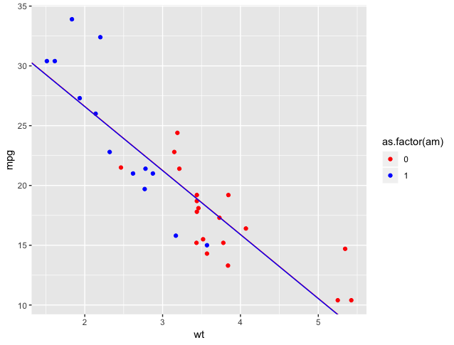 

anova(my_multi_model_1)
anova(my_multi_model_2)

> anova(my_multi_model_1)
Analysis of Variance Table

Response: mpg
              Df Sum Sq Mean Sq F value    Pr(>F)    
wt             1 847.73  847.73 88.3302 2.645e-10 ***
as.factor(am)  1   0.00    0.00  0.0002    0.9879    
Residuals     29 278.32    9.60                      
---
Signif. codes:  0 ‘***’ 0.001 ‘**’ 0.01 ‘*’ 0.05 ‘.’ 0.1 ‘ ’ 1
> anova(my_multi_model_2)
Analysis of Variance Table

Response: mpg
              Df Sum Sq Mean Sq F value    Pr(>F)    
as.factor(am)  1 405.15  405.15  42.215 4.110e-07 ***
wt             1 442.58  442.58  46.115 1.867e-07 ***
Residuals     29 278.32    9.60                      
---
Signif. codes:  0 ‘***’ 0.001 ‘**’ 0.01 ‘*’ 0.05 ‘.’ 0.1 ‘ ’ 1

> Anova(my_multi_model_1)
Anova Table (Type II tests)

Response: mpg
              Sum Sq Df F value    Pr(>F)    
wt            442.58  1 46.1151 1.867e-07 ***
as.factor(am)   0.00  1  0.0002    0.9879    
Residuals     278.32 29                      
---
Signif. codes:  0 ‘***’ 0.001 ‘**’ 0.01 ‘*’ 0.05 ‘.’ 0.1 ‘ ’ 1
> Anova(my_multi_model_2)
Anova Table (Type II tests)

Response: mpg
              Sum Sq Df F value    Pr(>F)    
as.factor(am)   0.00  1  0.0002    0.9879    
wt            442.58  1 46.1151 1.867e-07 ***
Residuals     278.32 29                      
---
Signif. codes:  0 ‘***’ 0.001 ‘**’ 0.01 ‘*’ 0.05 ‘.’ 0.1 ‘ ’ 1

Interaction Effects

Fine, so it looks like transmission type alone doesn’t have much predictive power (it has a very high p value). But I do think there’s something going on with transmission type. Let me model mpg as a function of the interaction between weight and transmission type. In other words, I think that transmission type influences the relationship between weight and mpg.

We can calculate this as mpg ~ weight + as.factor(am) + wt:as.factor(am), where we use a colon (:) to indicate interaction, or, much more simply, using a “cross”, indicated in our formula by *:

my_multi_model_4 <- lm(mpg ~wt*as.factor(am), mtcars)
summary(my_multi_model_4)

The model above gives us the following output:

> summary(my_multi_model_4)

Call:
lm(formula = mpg ~ wt * as.factor(am), data = mtcars)

Residuals:
    Min      1Q  Median      3Q     Max 
-3.6004 -1.5446 -0.5325  0.9012  6.0909 

Coefficients:
                  Estimate Std. Error t value Pr(>|t|)    
(Intercept)        31.4161     3.0201  10.402 4.00e-11 ***
wt                 -3.7859     0.7856  -4.819 4.55e-05 ***
as.factor(am)1     14.8784     4.2640   3.489  0.00162 ** 
wt:as.factor(am)1  -5.2984     1.4447  -3.667  0.00102 ** 
---
Signif. codes:  0 ‘***’ 0.001 ‘**’ 0.01 ‘*’ 0.05 ‘.’ 0.1 ‘ ’ 1

Residual standard error: 2.591 on 28 degrees of freedom
Multiple R-squared:  0.833,	Adjusted R-squared:  0.8151 
F-statistic: 46.57 on 3 and 28 DF,  p-value: 5.209e-11

The output from this summary is trickier to interpret (but promises to pay off, as we see a very good R-squared). We know that am has two values, 0 and 1, and we see that two of our coefficients list am of 1, so those two coefficients are for when am = 1. But how do I use these coefficients to calculate a prediction or draw a line?

We’ll go one at a time:

• (Intercept) is the base y-intercept, assuming am of 0.
• wt is the slope of a line, assuming am of 0.
• as.factor(am)1 is the additional intercept added when am = 1.
• wt:as.factor(am)1 is the additional slope added when am = 1.

So, we have two lines:

• When am = 0: $mpg=-3.7859\cdot{wt}+31.4161$
• When am = 1: $mpg=-9.084268\cdot{wt}+46.29448$

Let’s plot!

ggplot(mtcars, aes(wt, mpg)) +
  geom_point(aes(color=as.factor(am))) +
  scale_color_manual(values=c("red", "blue")) +
  geom_abline(intercept = my_multi_model_4$coefficients[1], 
              slope = my_multi_model_4$coefficients[2], 
              color = "red") +
  geom_abline(intercept = my_multi_model_4$coefficients[1] +
                          my_multi_model_4$coefficients[3], 
              slope = my_multi_model_4$coefficients[2]+
                      my_multi_model_4$coefficients[4], 
              color = "blue")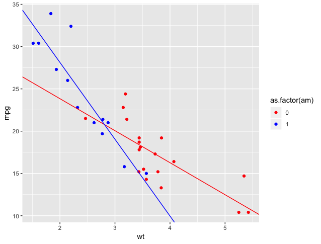

Much better!

Interaction terms without main effects?

What happens if you specify a model with only an interaction term and no main effects, for example, mpg ~ wt:as.factor(am)? The answer is that it depends on the variables in your model.

If you have only categorical predictors, then most statistical software (including R) will just reparameterize the full model with main effects and interactions if you try to run an interaction-only model. That means the underlying math will be the same, and all of the model fit statistics etc. will be identical whether you include the main effects or not. What changes is the estimates of the regression coefficients, because the model will shift the reference group represented in the intercept. Nothing meaningful about the model changes, though.

If you have any continuous predictors, though, then omitting main effects when you put in an interaction will almost always result in a misspecified model. That means the model isn’t actually estimating what you mean it to estimate, and any model results are meaningless. In our case, if we ran mpg ~ wt:as.factor(am), it would force R to estimate only one intercept for both levels of am, which will pull the best fit lines away from the data they should describe. The reverse situation, where you have only main effects and no interaction is much easier to interpret — we estimate a different intercept for each am group, but we assume the effect of wt on mpg is the same regardless (i.e. only one slope), so we’re looking at parallel lines. That may or may not actually make theoretical sense (do you really think the effect of wt on mpg is independent of am?), but at least it’s interpretable. When we include both main effects and the interaction, we estimate a separate intercept and slope for each am group, which is again pretty interpretable.

But when we estimate only an interaction with no main effects, then we force both lines to go through the same intercept, and that means the slopes we get for each am group will also be very weird — once you force a regression line to go through a particular point, then the only way it can get closer to its data points (every regression line’s dearest wish) is by adjusting its slope, which means you might get more extreme slope estimates than are actually justified by the data. You can see that happening in the plot below, which shows regression lines from both a full model (including both main effects and the interaction) and from a model with the interaction alone, plotted separately for the two groups of am. As you can see in am=0, the interaction-only model estimates an intercept that’s too high for that group, and the resulting line has to slope down sharply in order to reach its data; the reverse happens in am=1. The estimated slopes for the effect of wt therefore describe neither the separate am groups (as they do in the full model), nor the data pooled across both am groups (as they do in the main effects model).

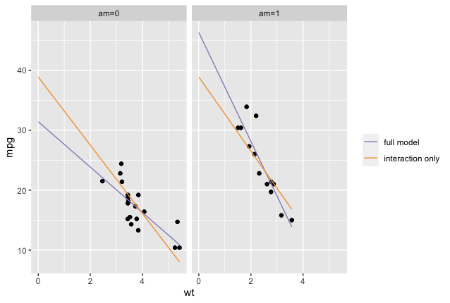
To sum up, while it is mathematically possible to estimate interaction-only models, it’s generally not a good idea.

For more on interaction-only models, see this post.

Conclusions

• You can use lm to come up with a fast linear model for a single predictor or multiple predictors.
• You can combine multiple predictors with “+” (add a main effect), “:” (add an interaction effect), or “*” (add main effects and an interaction effect).
• Check your solution both visually (graph it) and statistically (read the output of summary()).

So far, we’ve assumed you knew ahead of time what variables to use to construct your model. But sometimes you might have 50 variables available to you, with no clear hypothesis about which ones to use. You want to use enough information to get a close prediction, but not so much that the model is nearly impossible to use in the real world. In an upcoming article, we’ll talk about how to get a linear model in these conditions, by choosing the most predictive sets of variables.