
R 4 Beginners Chapter 7 - Reading Tabular Data
R 4 Beginners
An exploration of data science as taught in R for Data Science by Hadley Wickham and Garrett Grolemund. This blog is meant to be a helpful addition to your own journey through the book. No prior programming experience necessary!
Chapter 7: Reading Tabular Data
Now that we’ve covered some of the basics of R programming, I might start combining some topics and sometimes presenting some things out of order. The information here is essentially a “highlight reel” that I hope is a quick way to get you started using R, but I highly recommend reading R4DS as you have the time– there will be much more detail in the book itself than I will go into here!
Reading in data
So far, we’ve been working with data that comes pre-packaged with the tidyverse or another package, but those datasets are just for practice, so we need to learn how to bring data into R from external sources. Data can come from a variety of places: you can type it in manually (which is error-prone, and frequently not even feasible), pulled from a database (BigQuery, in the Google ecosystem, is one example of a SQL database), scraped from a website… There are lots of places where data live! The simplest scenario, and one that is luckily quite common, is that you have tabular data in a file (such as a CSV or an Excel spreadsheet) that you need to import into R for analysis.
readr
Base R (the R you use if you haven’t loaded any other packages) has functions to read lots of different kinds of files, but the tidyverse has its own versions in the readr package. The readr versions are frequently faster and more reproducible than the base R versions (since they aren’t inheriting any behavior from your operating system, like base R can). The import functions in the tidyverse also have the added benefit of creating “tibbles”, the specific type of data frame used by the tidyverse, so you’ll have less work to do after data import if you are using the tidyverse for analysis or plotting (if you are interested in tibbles and how their behavior differs from a data.frame generated by base R, I recommend reading about it in Chapter 10 of R4DS). Which function you’ll want to use will depend on what kind of flat file you have (such as read_fwf() for fixed width files and read_tsv() for tab delimited files), but one of the most common is read_csv() for reading in comma delimited files. What all of these file formats have in common is that they are methods of storing tabular data in a plain text format; we’re used to seeing tabular data stored in spreadsheet programs such as Excel, but files like CSVs don’t require special software (check out this article to read more about flat file storage).
As an aside, it’s generally good practice to store files in plain text when you can. I know I’ve certainly felt the pain of trying to open a really old Excel file in a newer version of the software, only to end up with data that are totally corrupted. You can use Excel to open CSV files (and save your Excel files as CSVs) so it’s a good habit to get into. To read more about using spreadsheets (and, more to the point, when it might be a better idea not to) check out this article about Excel caveats and its sequel.
File parsing
Part of what makes readr so powerful is that when you give it a file to read, it makes educated guesses about what kind of data each column contains– this is a process called parsing. There are a group of parsing functions that can be run on vectors essentially to examine what kind of values they may contain, such as characters (like “abc”), integers, decimals, logicals (like TRUE or FALSE), and many more. If you are interested in how the tidyverse parses vectors, definitely read more about it here in R4DS; it’s an interesting topic. Mostly what you need to know is that readr uses some heuristics to guess what parser it should use for each column based on what values it finds in the first 1000 rows and then parses the rest of the column based on this guess.
Let’s look at example. Let’s say that I’m a researcher studying the levels of Enzyme X in my (completely made-up) study population. In a spreadsheet I’ve recording the date of the experiment (“exp_date”), the dates of birth of these study participants (“dob”), and their blood levels of Enzyme X (“x_levels”). If I import that CSV into R using readr by running the code enzyme_x_levels <- read_csv("enzyme_x.csv") and take a look at it (with head(enzyme_x_levels)), I’ll see something like this:
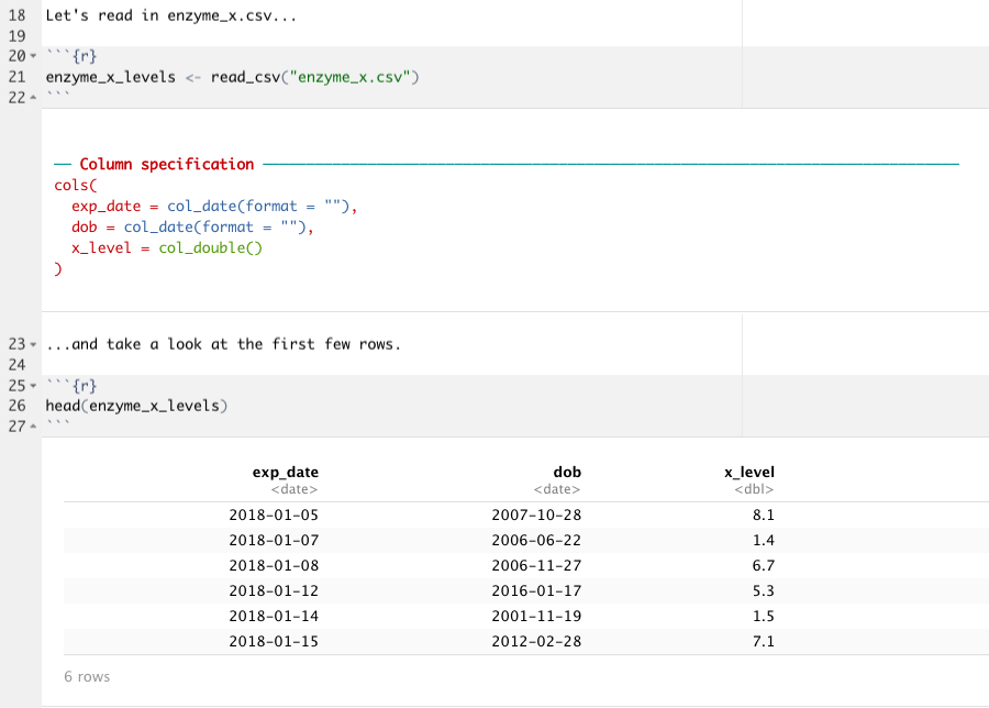
Notice that below your code chunk you’ll see that read_csv() is giving you the data type that it guessed for each column; the exp_date and dob columns are both dates, and the x_level column contains doubles (in other words, decimal numbers). This automatic parsing means that the values in each column are formatted correctly, and that we can go head and do calculations with the numerical column, or anything we need to do with the dates, without having to tell readr what kinds of values are in each column.
There are a few ways that this parsing can fail, however. If for some reason the first 1000 rows are special cases (if, for instance, the way the data were recorded changed over time), or there is a lot of missing data, the parsing can fail. The function problems() can help identify where these failures are occurring. What if as I was researching Enzyme X, I discovered some time later that Enzyme Y might also be involved in the effect that I am studying, and so I start taking Enzyme Y levels. However, for most experimental days, I still only have Enzyme X levels. Let’s look at what I might see if I read in my new CSV:
enxymes_xy_levels <- read_csv("enzymes_xy.csv")
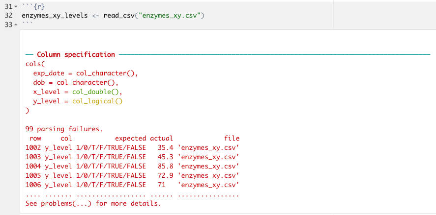
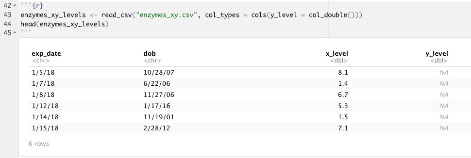
What you can see here is that readr has warned me that there were 99 parsing failures when I tried to import my CSV of Enzyme X and Enzyme Y values; it looks like read_csv() thought that column y_level was a logical value, not a double! If I take a look at my data, I suspect that I know why. Because the first 1001 rows do not contain any data for y_level, read_csv() didn’t even look at the rest of the values; instead, it just made the best guess with the data in the first 1000 rows which all contain NA. If we can figure out from looking at the data what the column type should be, which we can in this case (we know the column specification should be double, just like x_level) we can use the argument col_types in the read_csv() function (or other readr functions) to specify exactly what each column type should be. This process uses functions that take the form col_*():
enzymes_xy_levels <- read_csv("enzymes_xy.csv",
                      col_types = cols(y_level = col_double()))
There are quite a few arguments in the readr functions besides col_types so I recommend looking through the documentation to get all of the details. If you would like to practice using read_csv() and parsing columns, check out R4DS here. It goes through a sample dataset in readr called “challenge.csv” that you can bring in by running read_cvs(readr_example("challenge.csv")) that is designed to fail with default parsing– play around with it! There is also a handy cheatsheet for importing data with readr, as well as working with the tibbles that it creates. It also gives some information about writing to delimited files.
Writing to a file
Just like you can read in a CSV file to create a tibble, you can take a tibble and write a new CSV file (or other kind of file). The function is write_csv() (or write_delim(), write_tsv(), or write_excel_csv()), and all you need is the name of the tibble and a file path where you’d like to save it. Let’s say, for example, I used the dplyr mutate() function (remember that from chapter 5 of this series?) to calculate a new column with the ratio of Enzyme X to Enzyme Y, and I wanted to save the new table as a separate CSV. I could use the write_csv() function to do that:
xy_ratio <- mutate(enxymes_xy_levels, ratio = (x_level / y_level))
write_csv(xy_ratio, "xy_ratio.csv")
One caveat is that by saving this new tibble as a CSV, R won’t “remember” that I wanted the y_level column to be a double. If I ever import my new file “xy_ratio.csv” again, I’ll need to tell read_csv() to read y_level and ratio as double. If I did want to save the data types from my tibble, I could have saved it in a custom binary format in R called an RDS file with write_rds(xy_ratio, "xy_ratio.rds").
Other data sources
Sometimes you might not be using data that is stored as a CSV. Sometimes you’ll be using an Excel file, or retrieving data from a database, or pulling data from statistical analysis software such as SPSS or Stata. There are packages in the tidyverse or in the wider word of R that handle these types of data as well! You can use haven for SPSS or Stata, readxl for .xls and .xlsx Excel files, DBI for pulling from a database, jsonlite for JSON files, or xml2 for XML. In short, if you have data, R can read it somehow!