
ANOVA tables in R
I don’t know what fears keep you up at night, but for me it’s worrying that I might have copy-pasted the wrong values over from my output. No matter how carefully I check my work, there’s always the nagging suspicion that I could have confused the contrasts for two different factors, or missed a decimal point or a negative sign.
Although I’m usually overreacting, I think my paranoia isn’t completely misplaced — little errors are much too easy to make, and they can have horrifying consequences.
Through the years, I’ve learned that the only sure way to reduce human error is to give humans (including myself) as little opportunity to interfere in the process as possible. Happily, R integrates beautifully with output documents, allowing you to ask the computer to fill in the numbers in your tables and text for you, so you never have to wake up in a cold sweat panicking about a typo in your correlation matrix. These are called dynamic documents, and they’re awesome.
I almost never type out my results anymore; I let R do it for me. I wrote my entire dissertation in R Studio, in fact, using sweave to integrate my R code with LaTeX typesetting. I’m writing this post in R Studio as an R-markdown document.
Even if you’ve never used markdown or R-markdown before, you can jump right in and start getting properly formatted output from R. In this tutorial, I’ll cover examples for one common model (an analysis of variance, or ANOVA) and show you how you can get table and in-line output automatically.
We’ll use one of the most basic functions for creating tables, kable, which is from one of the most user-friendly packages for combining R code and output together, knitr. (Side note to the fiber enthusiasts: Yes, you’re not imagining it — pretty much all of this stuff is playfully named after yarn, knitting, and textile references. Enjoy.) I recommend knitr and kable for people just getting into writing dynamic documents (also called literate statistical programming) because they’re the easiest and most flexible tools, especially since they can be used to create Word documents (not just pdfs or html pages). Depending on your desired output, though, you may find other packages better suited to your needs. For example, if you’re creating pdf documents, you may prefer pander, xtable or stargazer, all of which are much more powerful and elegant. Although these are excellent packages, I find they don’t work consistently (or at all) for Word output, which is a deal breaker for a lot of people.
Quick links to content in this tutorial:
Creating an APA style ANOVA table from R output
A quick note: I’m using APA style results for the examples here because that’s my background. APA style is also particularly demanding and nit-picky, so conforming to APA standards is a good exercise for showing customization options. The code here can be adapted for pretty much any formatting you need, though, so feel free to take what works for you and leave the rest.
This tutorial assumes…
- That you are using R Studio. If you don’t have it already, it’s free to downloada and install, just like R.
- That you already have a basic understanding of what an ANOVA is and when you might use it.
- That you’re not brand new to R. If you are, the descriptions may still be useful to you, but you may run into problems replicating the analysis on your own computer or editing the code to suit your needs.
Running an ANOVA in R
Set up
Since the kable function is part of the knitr package, you’ll need to load knitr before you can use it:
library(knitr)
We’ll use a data set that comes built into R: warpbreaks. Fittingly, it’s about yarn. It gives the number of breaks in yarn tested under conditions of low, medium, or high tension, for two types of wool (A and B). This data comes standard with R, so you already have it on your computer. You can read the help documentation about this data set by typing ?warpbreaks in the console.
str(warpbreaks) # check out the structure of the data
We’ll run a 2x3 factorial ANOVA to test if there are differences in the number of breaks based on the type of wool and the amount of tension.
Exploratory data analysis
Before running a model, you always want to plot the data, to check that your assumptions look okay. Here are a couple plots I might generate while analyzing these data:
library(ggplot2)
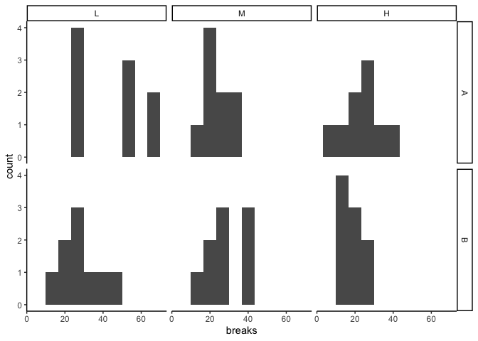
# histograms, to check out the distribution within each group
ggplot(warpbreaks, aes(x=breaks)) +
geom_histogram(bins=10) +
facet_grid(wool ~ tension) +
theme_classic()
# boxplot, to highlight the group means
ggplot(warpbreaks, aes(y=breaks, x=tension, fill = wool)) +
  geom_boxplot() +
  theme_classic()
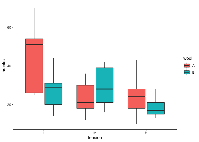
The box plot gives me an idea of what I might find in the ANOVA. It looks like there are differences between groups, with fewer breaks at higher tension, and perhaps fewer breaks in wool B vs. wool A at both low and high tension.
The distributions within each cell look pretty wonky, but that’s not particularly surprising given the small sample size (n=9):
xtabs(~ wool + tension, data = warpbreaks)

##     tension
## wool L M H
##    A 9 9 9
##    B 9 9 9
Running the model
One important consideration when running ANOVAs in R is the coding of factors (in this case, wool and tension). By default, R uses traditional dummy coding (also called “treatment” coding), which works great for regression-style output but can produce weird sums of squares estimates for ANOVA style output.
To be on the safe side, always use effects coding (contr.sum) or orthogonal contrast coding (e.g. contr.helmert, contr.poly) for factors when running an ANOVA.
Here, I’m choosing to use effects coding for wool, and polynomial trend contrasts for tension.
model <- lm(breaks ~ wool * tension,
            data = warpbreaks,
            contrasts = list(wool = "contr.sum", tension = "contr.poly"))
Annotated ANOVA output
The output you’ll want to report for an ANOVA depends on the motivation for running the model (is it the main hypothesis test for your study, or just part of the preliminary descriptive stats?) and the reporting conventions for the journal you intend to submit to. In many cases, you will only want to report the means and standard deviations for each cell with notes indicating which main effects and interactions are significant, and skip reporting the full ANOVA results. Here, I’m going to assume the ANOVA model is central to your research question, though, so we can see what a full and detailed report might look like. APA style includes specific guidelines for reporting ANOVA models, which is what I’m using here.
APA style ANOVA tables generally include the sums of squares, degrees of freedom, F statistic, and p value for each effect. You can get all of those calculations with the Anova function from the car package. It’s important to use the Anova function rather than the summary.aov function in base R because Anova allows you to control the type of sums of squares you want to calculate, whereas summary.aov only uses Type 1 (generally not what you want, especially if you have an unblanced design and/or any missing data).
library(car)

## Loading required package: carData

sstable <- Anova(model, type = 3) # Type III sums of squares is standard, in the social sciences at least

sstable

## Anova Table (Type III tests)
##
## Response: breaks
##              Sum Sq Df  F value    Pr(>F)
## (Intercept)   42785  1 357.4672 < 2.2e-16 ***
## wool            451  1   3.7653 0.0582130 .
## tension        2034  2   8.4980 0.0006926 ***
## wool:tension   1003  2   4.1891 0.0210442 *
## Residuals      5745 48
## ---
## Signif. codes:  0 '***' 0.001 '**' 0.01 '*' 0.05 '.' 0.1 ' ' 1
The above code runs the Anova function on the model I saved before, using Type III sums of squares, and saves the resulting table as a new object called sstable.
In sstable, you can see a row for each predictor in the model, including the intercept, and the error term (Residuals) at the bottom. The wool:tension term is the interaction between wool and tension (R uses : to specify interaction terms, and * as shorthand for an interaction term with both main effects). There are two levels of wool (A and B), so you’ll see 1 degree of freedom for that effect. There are three levels of tension (low, medium, and high), so that has 2 degrees of freedom. The interaction has the df for both terms multiplied together, i.e. 1 * 2 = 2.
The degrees of freedom for the residual are based on the total number of observations in the data (N=54) minus the number of groups, i.e. 54-6=48.
The F-statistic for each effect is the SS*/*df for that effect divided by the SS*/*df for the residual. The Pr(>F) gives the p value for that test, i.e. the probability of observing an F ratio greater than that given the null hypothesis is true.
Contrast estimates
summary.aov(model, split = list(tension=list(L=1, Q=2)))

##                   Df Sum Sq Mean Sq F value   Pr(>F)
## wool               1    451   450.7   3.765 0.058213 .
## tension            2   2034  1017.1   8.498 0.000693 ***
##   tension: L       1   1951  1950.7  16.298 0.000194 ***
##   tension: Q       1     84    83.6   0.698 0.407537
## wool:tension       2   1003   501.4   4.189 0.021044 *
##   wool:tension: L  1    251   250.7   2.095 0.154327
##   wool:tension: Q  1    752   752.1   6.284 0.015626 *
## Residuals         48   5745   119.7
## ---
## Signif. codes:  0 '***' 0.001 '**' 0.01 '*' 0.05 '.' 0.1 ' ' 1
(Note that if you run summary(model) instead, you’ll get the default regression-style output, which is the same information, but represented as regression coefficients with standard errors and t-tests instead of sums of squares estimates with F ratios.)
What we see here is a significant linear trend in the main effect for tension — from the box plot we made before, we know that it’s a negative linear trend. There’s no overall quadratic trend in tension, but there is a quadratic trend in the interaction between wool and tension. That means the estimate of the quadratic trend contrast is different for wool A compared to wool B. Referencing the box plot again, you can see that the direction of the quadratic trend appears to differ in wool A compared to wool B (wool A looks like a positive quadratic trend, with an upward swoop, whereas wool B looks like a negative quadratic trend, with an upside-down U swoop). There is no linear trend for the interaction, however, so that the estimate of the linear trend in wool A is not significantly different from the estimate of the linear trend in wool B.
Remember that summary.aov is using Type I sums of squares, so the estimates for some effects may not be what we want. In this example, the design is balanced and there are no missing data, so the SS estimates using Type I and Type III work out to be the same, but in your own data there may be a difference.
Note that our orthogonal contrasts here are simple comparisons between means, and aren’t affected by the type of SS used. If you are concerned about Type of SS, you may want to grab the contrast estimates from this output and put them into your other sstable object. Here’s how you could do that:
Note which rows in the output correspond to the contrasts you want. In this case, it’s rows 3 and 4 for the contrasts on the main effect of tension, and rows 6 and 7 for the contrasts on the interaction. I select those rows with c(3, 4, 6, 7). I’m also selecting and reordering the columns in the output, so they’ll match what we have in sstable. I select the 2nd column (Sum Sq), then the first (Df), then the fourth (F value), then the fifth (Pr(>F)) with c(2, 1, 4, 5).
Remember that you can use [ , ] to select particular combinations of rows and columns from a given matrix or dataframe. Just put the rows you want as the first argument, and the columns as the second, i.e. [r, c]. If you leave either the rows or the columns blank, it will return all (so [r, ] will return row r and all columns).
# this pulls out just the specified rows and columns
contrasts <- summary.aov(model, split = list(tension=list(L=1, Q=2)))[[1]][c(3, 4, 6, 7), c(2, 1, 4, 5)]

contrasts

##                    Sum Sq Df F value    Pr(>F)
##   tension: L      1950.69  1 16.2979 0.0001938 ***
##   tension: Q        83.56  1  0.6982 0.4075366
##   wool:tension: L  250.69  1  2.0945 0.1543266
##   wool:tension: Q  752.08  1  6.2836 0.0156262 *
## ---
## Signif. codes:  0 '***' 0.001 '**' 0.01 '*' 0.05 '.' 0.1 ' ' 1
Now use rbind to create a sort of Frankenstein table, splicing the contrasts estimate rows in with the other rows of sstable.
# select the rows to combine
maineffects <- sstable[c(1,2,3), ]
me_contrasts <- contrasts[c(1,2), ]
interaction <- sstable[4, ]
int_contrasts <- contrasts[c(3,4), ]
resid <- sstable[5, ]

# bind the rows together in the desired order
sstable <- rbind(maineffects, me_contrasts, interaction, int_contrasts, resid)

sstable # ta-da!

## Anova Table (Type III tests)
##
## Response: breaks
##                   Sum Sq Df  F value    Pr(>F)
## (Intercept)        42785  1 357.4672 < 2.2e-16 ***
## wool                 451  1   3.7653 0.0582130 .
## tension             2034  2   8.4980 0.0006926 ***
##   tension: L        1951  1  16.2979 0.0001938 ***
##   tension: Q          84  1   0.6982 0.4075366
## wool:tension        1003  2   4.1891 0.0210442 *
##   wool:tension: L    251  1   2.0945 0.1543266
##   wool:tension: Q    752  1   6.2836 0.0156262 *
## Residuals           5745 48
## ---
## Signif. codes:  0 '***' 0.001 '**' 0.01 '*' 0.05 '.' 0.1 ' ' 1
Estimates of effect size
A popular measure of effect size for ANOVAs (and other linear models) is partial eta-squared. It’s the sums of squares for each effect divided by the error SS. The following code adds a column to the sstable object with partial eta-squared estimates for each effect:
sstable$pes <- c(sstable$'Sum Sq'[-nrow(sstable)], NA)/(sstable$'Sum Sq' + sstable$'Sum Sq'[nrow(sstable)]) # SS for each effect divided by the last SS (SS_residual)

sstable

## Anova Table (Type III tests)
##
## Response: breaks
##                   Sum Sq Df  F value  Pr(>F)     pes
## (Intercept)        42785  1 357.4672 0.00000 0.88162
## wool                 451  1   3.7653 0.05821 0.07274
## tension             2034  2   8.4980 0.00069 0.26149
##   tension: L        1951  1  16.2979 0.00019 0.25348
##   tension: Q          84  1   0.6982 0.40754 0.01434
## wool:tension        1003  2   4.1891 0.02104 0.14861
##   wool:tension: L    251  1   2.0945 0.15433 0.04181
##   wool:tension: Q    752  1   6.2836 0.01563 0.11576
## Residuals           5745 48
Okay great! There’s your output, but you don’t want to just copy-paste that mess into your manuscript. Let’s get R to generate a nice, clean table we can use in Word.
Creating an APA style ANOVA table from R output
kable(sstable, digits = 3) # the digits argument controls rounding
| Sum Sq | Df | F value | Pr(>F) | pes | |
|---|---|---|---|---|---|
| (Intercept) | 42785.185 | 1 | 357.467 | 0.000 | 0.882 |
| wool | 450.667 | 1 | 3.765 | 0.058 | 0.073 |
| tension | 2034.259 | 2 | 8.498 | 0.001 | 0.261 |
| tension: L | 1950.694 | 1 | 16.298 | 0.000 | 0.253 |
| tension: Q | 83.565 | 1 | 0.698 | 0.408 | 0.014 |
| wool:tension | 1002.778 | 2 | 4.189 | 0.021 | 0.149 |
| wool:tension: L | 250.694 | 1 | 2.095 | 0.154 | 0.042 |
| wool:tension: Q | 752.083 | 1 | 6.284 | 0.016 | 0.116 |
| Residuals | 5745.111 | 48 | NA | NA | NA |
Wait, what? That was so easy!
Yes, yes it was. :)
In a lot of cases, that will be all you need to get a workable ANOVA table in your document. Just for fun, though, let’s play around with customizing it a little.
Hide missing values
By default, kable displays missing values in a table as NA, but in this case we’d rather have them just be blank. You can control that with the options command:
options(knitr.kable.NA = '') # this will hide missing values in the kable table

kable(sstable, digits = 3)
| Sum Sq | Df | F value | Pr(>F) | pes | |
|---|---|---|---|---|---|
| (Intercept) | 42785.185 | 1 | 357.467 | 0.000 | 0.882 |
| wool | 450.667 | 1 | 3.765 | 0.058 | 0.073 |
| tension | 2034.259 | 2 | 8.498 | 0.001 | 0.261 |
| tension: L | 1950.694 | 1 | 16.298 | 0.000 | 0.253 |
| tension: Q | 83.565 | 1 | 0.698 | 0.408 | 0.014 |
| wool:tension | 1002.778 | 2 | 4.189 | 0.021 | 0.149 |
| wool:tension: L | 250.694 | 1 | 2.095 | 0.154 | 0.042 |
| wool:tension: Q | 752.083 | 1 | 6.284 | 0.016 | 0.116 |
| Residuals | 5745.111 | 48 |
Add a table caption
You can add a title for the table if you change the format to “pandoc”. Depending on your final document output (pdf, html, Word, etc.), you can get automatic table numbering this way as well, which saves much time and many headaches.
kable(sstable, digits = 3, format = "pandoc", caption = "ANOVA table")
| Sum Sq | Df | F value | Pr(>F) | pes | |
|---|---|---|---|---|---|
| (Intercept) | 42785.185 | 1 | 357.467 | 0.000 | 0.882 |
| wool | 450.667 | 1 | 3.765 | 0.058 | 0.073 |
| tension | 2034.259 | 2 | 8.498 | 0.001 | 0.261 |
| tension: L | 1950.694 | 1 | 16.298 | 0.000 | 0.253 |
| tension: Q | 83.565 | 1 | 0.698 | 0.408 | 0.014 |
| wool:tension | 1002.778 | 2 | 4.189 | 0.021 | 0.149 |
| wool:tension: L | 250.694 | 1 | 2.095 | 0.154 | 0.042 |
| wool:tension: Q | 752.083 | 1 | 6.284 | 0.016 | 0.116 |
| Residuals | 5745.111 | 48 |
ANOVA table
Modify column and row names
Often, the automatic row names and column names aren’t quite what you want. If so, you’ll need to modify them for the sstable object itself, and then run kable on the updated object.
colnames(sstable) <- c("SS", "df", "$F$", "$p$", "partial $\\eta^2$")

rownames(sstable) <- c("(Intercept)", "Wool", "Tension", "Tension: Linear Trend", "Tension: Quadratic Trend", "Wool x Tension", "Wool x Tension: Linear Trend", "Wool x Tension: Quadratic Trend", "Residuals")

kable(sstable, digits = 3, format = "pandoc", caption = "ANOVA table")
| SS | df | F | p | partial η2 | |
|---|---|---|---|---|---|
| (Intercept) | 42785.185 | 1 | 357.467 | 0.000 | 0.882 |
| Wool | 450.667 | 1 | 3.765 | 0.058 | 0.073 |
| Tension | 2034.259 | 2 | 8.498 | 0.001 | 0.261 |
| Tension: Linear Trend | 1950.694 | 1 | 16.298 | 0.000 | 0.253 |
| Tension: Quadratic Trend | 83.565 | 1 | 0.698 | 0.408 | 0.014 |
| Wool x Tension | 1002.778 | 2 | 4.189 | 0.021 | 0.149 |
| Wool x Tension: Linear Trend | 250.694 | 1 | 2.095 | 0.154 | 0.042 |
| Wool x Tension: Quadratic Trend | 752.083 | 1 | 6.284 | 0.016 | 0.116 |
| Residuals | 5745.111 | 48 |
ANOVA table
Omit the intercept row
For many models, the intercept is not of any theoretical interest, and you may want to omit it from the output. If you just want to drop one row (or column), the easiest approach is to indicate that row’s number and put a minus sign before it:
kable(sstable[-1, ], digits = 3, format = "pandoc", caption = "ANOVA table")
| SS | df | F | p | partial η2 | |
|---|---|---|---|---|---|
| Wool | 450.667 | 1 | 3.765 | 0.058 | 0.073 |
| Tension | 2034.259 | 2 | 8.498 | 0.001 | 0.261 |
| Tension: Linear Trend | 1950.694 | 1 | 16.298 | 0.000 | 0.253 |
| Tension: Quadratic Trend | 83.565 | 1 | 0.698 | 0.408 | 0.014 |
| Wool x Tension | 1002.778 | 2 | 4.189 | 0.021 | 0.149 |
| Wool x Tension: Linear Trend | 250.694 | 1 | 2.095 | 0.154 | 0.042 |
| Wool x Tension: Quadratic Trend | 752.083 | 1 | 6.284 | 0.016 | 0.116 |
| Residuals | 5745.111 | 48 |
ANOVA table
Inline APA-style output
You can also knit R output right into your typed sentences! To include inline R output, use back-ticks, like this:
Here's a sentence, and I want to let you know that the total number of cats I own is `r length(my_cats)`.
The back-ticks mark out the code to run, and the r after the first back-tick tells knitr that it’s R code (if you feel the need, you can incorporate code from pretty much any language you like, not just R). Assuming there’s a vector called my_cats, when we knit the document, that line of code will be evaluated and the result (the number of items in the vector my_cats) will be printed right in that sentence.
Let’s work this into our ANOVA reporting.
Here’s an example write-up of this ANOVA, using inline code to plug in the stats. Since the inline code can be a little hard to read, I like to save all of the variables I want to use inline with convenient names first.
fstat <- unname(summary(model)$fstatistic[1])
df_model <- unname(summary(model)$fstatistic[2])
df_res <- unname(summary(model)$fstatistic[3])
rsq <- summary(model)$r.squared
p <- pf(fstat, df_model, df_res, lower.tail = FALSE)
Then I can plug them in as needed in my writing.
A 2x3 factorial ANOVA revealed that wool type (A or B) and tension (low, medium, or high) predict a significant amount of variance in number of breaks, $R^2$=`r round(rsq, 2)`, $F(`r round(df_model, 0)`, `r round(df_res, 0)`)=`r round(fstat, 2)`$, $p=`r ifelse(round(p, 3) == 0, "<.001", round(p, 3))`$.
Here’s how that code renders when knit: A 2x3 factorial ANOVA revealed that wool type (A or B) and tension (low, medium, or high) predict a significant amount of variance in number of breaks, R2=0.38, F(5, 48) = 5.83, p = < .001.
Further Reading
You can use this strategy just to generate tables or little bits of output and then copy-paste them into your manuscript draft in Word (or wherever you write), and that will go a long way toward reducing the possibility for human error in your scientific writing. That’s a great way to get started, and if your own work habits (or those of your co-authors) rely strongly on MS tools that may be as far as you take it.
Once you start doing that, though, you’ll realize you still get caught in a trap where you have to remember to update all the output in your document every time you make a change in the data or analysis (e.g. your PI asks you to remove an outlier and re-run everything, so you painstakingly re-do every piece of output, then for the next draft she asks you to put the outlier back in and you have to check it all over again). The power of literate statistical programming and dynamic documents really comes through when you can write your whole document in the same environment you do your analysis (e.g. RStudio). Then, when you have an update, you can just change the one line of code at the top where, for example, you exclude that outlier or not, and when you “knit” the document all of the output will automatically update to reflect the change. It takes minutes instead of hours, and there’s no copy-pasting for you to accidentally mess up. Unlike with Word documents, R-markdown documents are plain text so they give you the option to take advantage of version control tools like git to keep rigorous records of all the changes made to both your analysis and your writing. Your entire change history is available to you in a tidy, transparent way, and you can even develop parallel versions of a document and then merge them down the road and never lose the history.
There are tons of great tools to help you write a huge range of content in R-markdown. Here are some specific references for popular formats and extensions:
- scientific manuscripts, including lots of ready templates that will match the formatting requirements for specific journals
- math expressions and equations
- citations and references, including automatic bibliographies
- presentation slides
- books, including easy application for ePub and Kindle formats
- blogs and websites
- online tutorials, including the option for interactive feedback
For more on creating tables using kable, as we did here, see this post. For more on inline R code, see this post. For a great general reference, see the RStudio cheatsheet for R-markdown. Note that if you open RStudio, you can access all of their excellent cheatsheets right there from the menu at the top: go to Help, then select Cheatsheets.