R 4 Beginners

An exploration of data science as taught in R for Data Science by Hadley Wickham and Garrett Grolemund. This blog is meant to be a helpful addition to your own journey through the book. No prior programming experience necessary!

Chapter 6: Reproducible Programming

In the previous chapters of this series, we have been writing all of our code in the console of RStudio. You probably know the drill by now: write a line of code, hit “Enter,” and hope you haven’t messed anything up. However, this isn’t the only way to write code, and actually isn’t the most common way. When working in RStudio, usually you will either be writing a script or creating an R Markdown document.

Scripts

Before we get into writing R scripts, let’s take another look at the layout of RStudio:

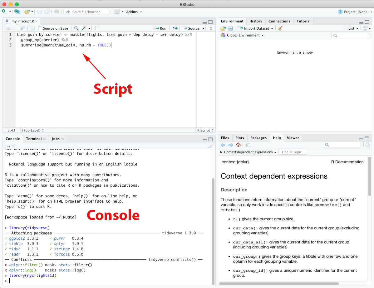
In this screenshot, you can see the console in the bottom left. In the top left quadrant is the editor, where you can write R scripts. You can open a new R script file in the “File” menu (there are several different file types you can choose, but “R Script” is probably the first option listed). The process of writing an R script is similar to writing code in the console, with a few key differences. The most important difference is that this is where you’ll write code that you want to save. There will be times that you want to save work you’ve been doing and come back to it later, or run the same code many times. In fact, if you close RStudio without saving your script it will reopen with the last script you were working on! It’s still good practice to save anything you definitely want to keep, of course, so try not to depend on that feature too much.

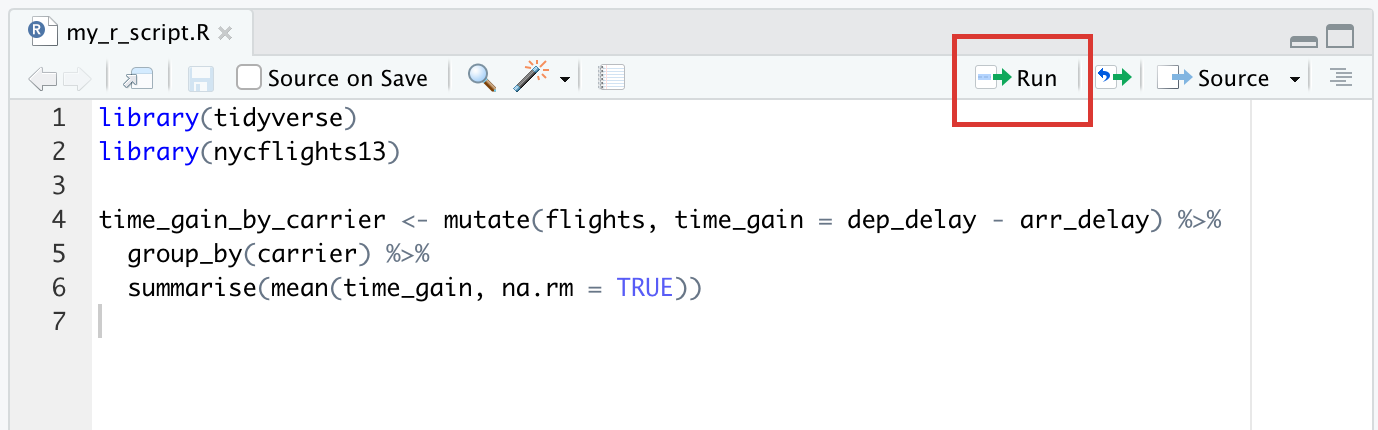
Another difference is that, previously, to run a line of code you would just hit the Enter/Return key. In a script, Enter/Return will take you to the next line (just like when you type in a word processor) rather than running the code you just wrote. This is a useful feature not only because it makes scripts easier to edit if you make a mistake, but also because it allows you to separate one code statement into several lines. When writing scripts, especially ones you want to come back to later or share with others, readability becomes quite important, and having parts of your code on multiple lines will help with that. To run a single code statement in a script, use Cmd/Ctrl + Enter; this will run the code where your cursor is, even if the code statement spans multiple lines like the script in the screenshot above, and then move the cursor to the next. If you have multiple code statements and you want to run all of them, you can highlight the block that you want to run and then hit Cmd/Ctrl + Enter. If you want to run the whole script, you can use the shortcut Cmd/Ctrl + Shift + S, or use the “Run” button at the top of the editor pane:

It’s usually a good idea to start scripts with loading the packages you’ll need, but it’s usually not a great idea to install packages in a script– it’s not generally useful, since you only need to install a package once, and if you’re sharing a script it’s not very considerate to install packages on someone else’s machine.

Comments

Scripts are a good way to write code that you want to keep, and following certain conventions can increase the readability of your code (here’s an article on the subject of making your code more readable), but sometimes it can just be difficult to tell exactly what a code statement is supposed to do. This is especially true if it has been a while since you wrote the code, or if you’re looking at someone else’s code. Luckily, there is a way to insert lines of text into your code, called comments. In many programming languages, including R, you mark comments with a pound sign (#). Marking comments lets your IDE (integrated development environment) know that the line that follows isn’t code and shouldn’t be run (which would certainly give you an error if it tried). Useful comments can include notes to yourself (about why you used a certain approach, a reminder of other things you tried first, etc.), notes to someone else explaining your reasoning, information about dependancies… the list goes on. Essentially, comments can be anything you want to say in actual words.

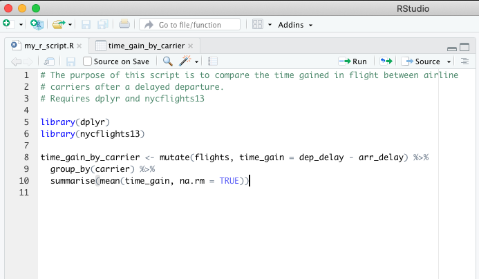
Here’s what comments can look like if you use them in a script:

R Markdown

If you’re following along in R4DS, you might notice that I’m about to go a bit out of order. R Markdown is one of the last topics that R4DS talks about, but it’s so useful that I wanted to talk about earlier. If you want to write your code in a truly reproducible way, R Markdown is an excellent way to do it. I think of R Markdown documents like entries in a scientific notebook– it’s not only a place to write and run code, but also where you write about your reasoning, organize your thoughts, and display visualizations and data. There are a couple of reasons that using R Markdown is an ideal method of reproducible programming:

1. In R Markdown, code chunks are interspersed with plain text. This might seem similar to commenting in a R script, except that you mark the code rather than the text– the text is the default. The difference may be subtle, but it changes how you think about writing code.

2. After an R Markdown document is written, it can then be knit into a nicely-formatted output document that can be HTML (the most common format), a Word document, a PDF, a scientific article, or one of a variety of other formats. This is useful for producing reports that are easily read and shared. With R Markdown your scientific reasoning, your code, and the output of your code can all be displayed in one easy-to-read format.

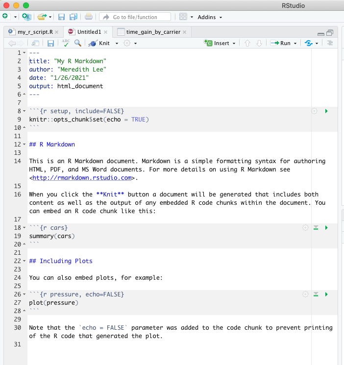
Let’s look at a simple example. When you open a new R Markdown file in RStudio, you’ll get some options to fill in before you even start. You’ll want to give it a title (you can always change this later) and choose your output format (HTML should be the default, you’ll need other packages to knit to other formats). Once you’ve done that, you’ll see that instead of a blank document, there’s stuff already on the page:

Before we dig into the details of R Markdown documents, I’ll mention that like so many aspects of working in RStudio, there’s a cheatsheet for R Markdown. There is also a handy R Markdown reference guide, which has a lot of the same content as the cheatsheet but is a little easier to read if you’re looking for syntax help.

Anatomy of an R Markdown Document

Text

Text in an R Markdown document doesn’t need to be marked, and is written in Markdown syntax (all of the articles on this site are actually written in Markdown!). Markdown is a way to add formatting to plaintext documents. If you want to learn more about Markdown (and you’ll need to if you want to create R Markdown documents, but I’m not going to go into it here), take a look at this guide to Markdown, which talks about the usefulness of Markdown as well as the basic syntax.

Code

In R Markdown, code chunks are surrounded by three backticks (```, you can see them in the R Markdown example above). Backticks are not the same as single quotes (though they can look similar in certain fonts); the backtick on your keyboard is likely in the upper left, on the same key as the tilde (~). Make sure you have the correct number of backticks, three before your code and three after, or strange things can happen (you’ll notice that RStudio makes the code chunks a different color to help you).

You’ll also need to tell RStudio that you are writing a chunk of R code by including {r} after the first set of backticks. This is because another cool thing about R Markdown files is that they can include code in other languages as well, including python, bash, and SQL. Beyond specifying the language of your code, there are other settings for code chunks:

• You can give your chunk a name with text right after the language ```{r chunk-name}, which can help with navigation to specific chunks (there’s a drop-down menu at the bottom-left of the editor).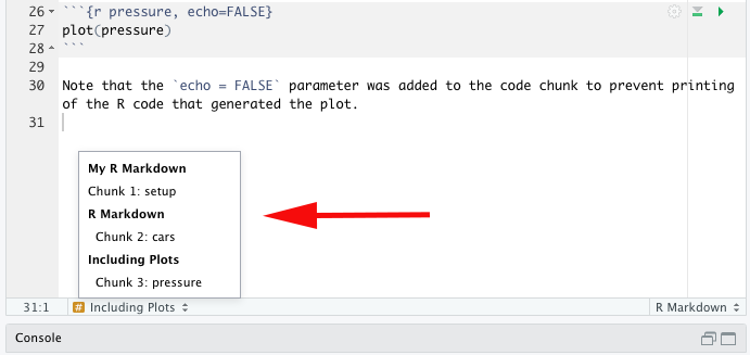 By the way, if you give your chunk the name “setup”, this chunk will run automatically before any other code. A setup chunk will already be there when you open a new R Markdown file, and will already have some code: knitr::opts_chunk$set(echo = TRUE). Whatever arguments you pass into knitr::opts_chunk$set() will be applied to every code chunk in the document unless you specify otherwise in individual chunks (in this case, echo = TRUE means that, by default, the actual code will be rendered in the knitted document, not just the output of the code).

• If you want a particular chunk of code to be hidden in the knitted document, and just want to see the output, you use would set up your chunk like this:

  ```{r echo = FALSE}
  YOUR CODE HERE
  ```
  

  This is a common setting for the setup code chunk. If instead you don’t want to see the code or the output, you would use include = FALSE (TRUE is the default). There are also settings like warning = FALSE or message = FALSE, which you can use to hide warnings and messages that RStudio gives you when your code runs.

YAML

The header at the top of an R Markdown document, surrounded by triple dashes (---), is written in a special language called “YAML”. Depending on who you ask, YAML stands for “YAML Ain’t Markup Language” or “Yet Another Markup Language”, but in the end, its purpose is to control certain aspects of the R Markdown document, especially pertaining to the way the output is displayed. As you can see in the example above, the YAML header can include the title, author, date of publication, and the output file type. These aren’t the only settings, but they’re a good starting place. Other options include:

• Parameters, which are values you can set once in the header that apply globally when the document renders (knits). For example, this could be useful if you want to create many reports that are all identical except for differences in a few key values. This field is called params. The params field is also the place that you can do cool things like use an R expression to automatically output the current date/time!

• You can also create a bibliography in the YAML header! You just need a bibliography file to link, and then R Markdown will append the citations in the file to the end of your output file after knitting.

Dashboards

There is a particularly useful, specialized type of R Markdown output called a dashboard. Dashboards are especially powerful when you want to show a group of related visualizations. Here is a great place to see a lot of good examples of dashboards! The dashboards in these examples were made using the flex_dashboard output, which you can use if you install and load the flexdashboard package. Once you’ve installed flexdashboard, RStudio will also give you the option of opening a flex dashboard template; when you open a new R Markdown file, go to “From Template” and select “Flex Dashboard”. You’ll see something that looks like this:

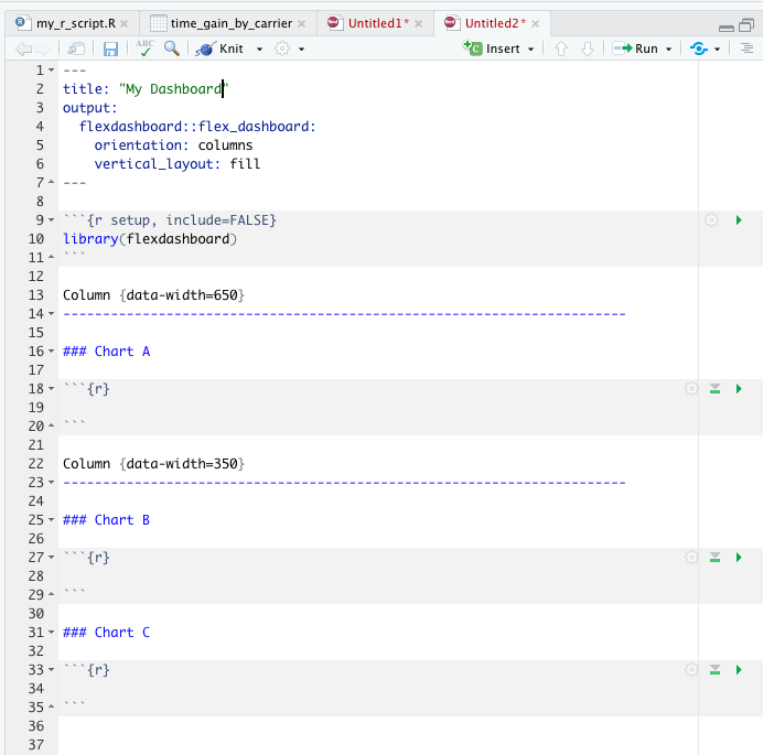
The process of writing text and code in your flex dashboard is the same as for a normal R Markdown document, except that now the document is divided into columns (or rows, if you change the orientation in the YAML header). This will change how the dashboard is displayed once knitted. There are lots of ways to customize dashboards, such as changing the general appearance by changing the theme, customizing the CSS (Cascading Style Sheets) styling, or adding a logo; all of these customizations are controlled in the YAML header. You can also make your dashboards interactive with plotly (a package for making ggplots interactive– the primary function is ggplotly()) and DT (a package for making tables interactive– the primary function is datatable()). To read more about interactivity in dashboards (and other HTML formats), check out htmlwidgets for R.

I’m not going to go into the details of all of the possible customizations for dashboards here, but just know there’s a lot that you can do! Here is a good place to start learning more about using and customizing flex dashboards.

Finally, you can get even more interactivity into your dashboards by hosting them as a Shiny app. This means that instead of JavaScript doing the work (which is what is happening when you use htmlwidgets), your R code is actually hosted on a Shiny server, and so the interactive elements are actually coming from the R code itself. Basically, in the static dashboard, the code is only run once and any interactivity is just the way it’s displayed using JavaScript, while in a Shiny app the actual code is changing and being re-run. This allows for things you can’t do with static dashboards, like responding to user input. You can learn more about Shiny apps here.

Projects

As you advance in your R journey, the time will come when what you want to accomplish will require more than just a single script. If you’re working on a project, you’ll want all of the files associated with that project in one convenient place all together. RStudio makes it simple to create new project directories and save files to them. When you want to start a project, instead of opening a new file, select “New Project…”. You’ll be asked if you want to start a new directory (which you can think of like a folder that holds your project files), associate it with an existing directory, or “checkout” a project from a version control repository like GitHub (for more info on version control, check out these resources). Whatever you select will become the working directory for your new project, and all of your scripts, R Markdown files, and any output files (such as visualizations and .csv files) will be stored there. This is very useful for a couple of reasons:

1. It keeps you organized! If you wrote code that yields a report as a PDF, you can find the report as well as the code that generated it right there in the same place.

2. It helps with collaboration. You can share a project and know that (pretty much) everything your collaborator needs is there in your project.

If you plan to share your project (and, really, it’s a good idea to write your code as if you might share it in the future), you’ll want to make sure that if your code contains files paths (like, for instance, if you are reading in data from a spreadsheet), it contains only relative file paths and no absolute file paths. This is important because the structure of a project means that everything is in the same working directory, so relative file paths are sufficient; if you use an absolute file path, the file path you would use on your computer won’t be the same as on someone else’s, because their home directory is different. Try running getwd(), which prints your current working directory, in your console or editor and you may see what I mean. Your username is probably in there, right? That will be different on a collaborator’s computer. But since you have everything in a project, you can use paths that are relative to the current working directory. If you want to read more about file paths, check out this article.

That concludes Part I of R 4 Beginners. If you are feeling a bit overwhelmed right now, that is totally normal! I felt the same way not so very long ago when I was getting started with R, and still do a lot of the time. There’s always so much to learn, but the best way to learn R is to use R! Get coding, even if it feels like you don’t know enough to start– you do. Before we get started on Part II, I’ll be posting some other types of content that will hopefully help you in your R journey, so stay tuned!