ggplot overview

Visualization with ggplot

ggplot2 (commonly referred to as just “ggplot”) allows you to make highly customizable graphics. It can provide publication-quality graphics that work perfectly for posters, publications, and simple sharing of your findings. “gg” stands for “the grammar of graphics”, and ggplot aims to apply some abstraction of visualization ideas into an understandable system. This results in a number of elements that together build up a graph.

For example, the “aesthetics” (aes) are data you can see on a graph. You might see, say, in the mtcars dataset, cyl (cylinders), wt (weight), and mpg (miles per gallon). We’re not saying yet just how you might see them – maybe you have a scatterplot where x = wt and y=mpg, and the cyl variable determines the size of the dot that’s on the scatterplot. Or maybe you might plot a graph for each kind of cyl – you have separate line plots that plot mpg by weight for each cylinder count. In this case, you’d have a graph for 4-cylinder cars, one for 6, and another for 8. You get the idea.

The main elements you need to consider are:

• data: what’s available to graph?
• aesthetic mapping: what part of the data is being graphed right now?
• geometric object: what kind of visualization will you have? Boxplot? Histogram? Scatterplot?

Additional elements could include:

• scales: do x and y need to have the same scale?
• faceting: do you want separate graphs by category?
• statistical manipulation: do you want to graph the mean of something?

You build up a ggplot graph by adding commands that enhance the plot – adding labels, titles, styling like color or font, graph elements like lines, points, or bars, and so forth. These commands are separated by plus signs.

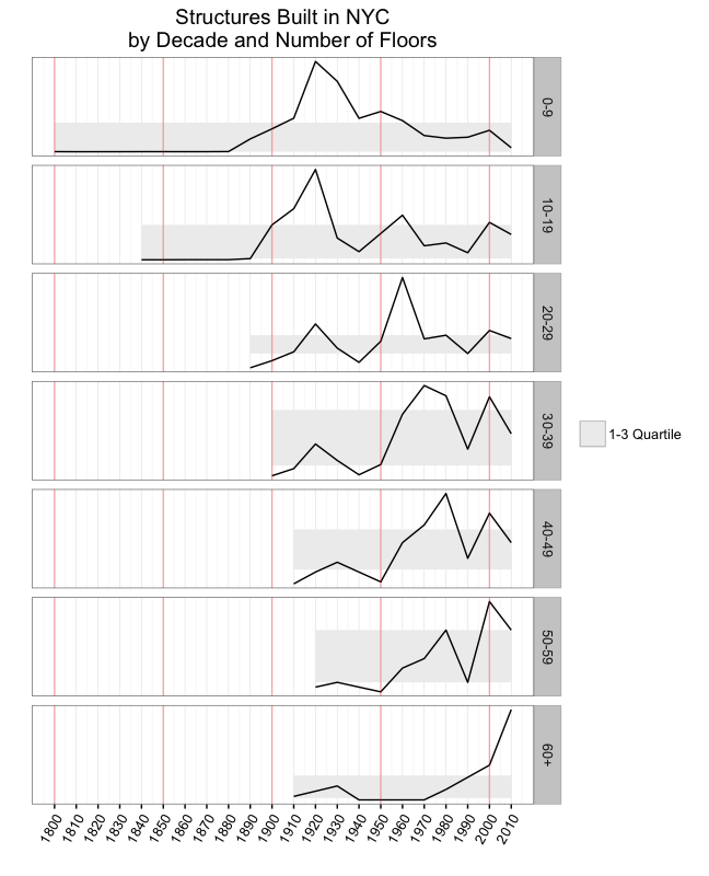
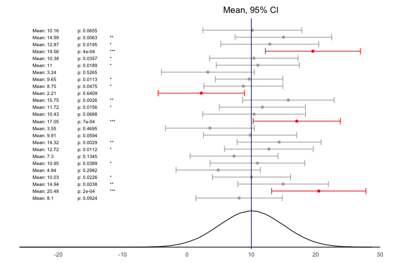
Here are a couple of complex graphs that I created using ggplot and wrote up in this website. Click the image to go to the article and see how I did it (the data is included, so you can follow along and do it as well!):

First plot: Sparklines!

Second plot: Confidence Intervals vs True Mean

These are pretty complex graphs, and while you’re welcome to start there, you might want to do something simpler instead to begin with. Let’s use the mtcars dataset as a way to do lots of different visualizations. You can follow along below, or download the complete code.

Plotting with mtcars

You start with something like plot <- (data_you_use, aes(elements_from_that_data_to_plot)). Nothing will plot just yet!

Before we go much further, let’s take a quick peek at mtcars. You’ll notice it’s in “wide” format – that is to say, every column is a variable and every row is an observation. The “wide” vs “long” data format will make sense later on, in posts where we deal with very complex data visualizations. Simple plots in ggplot don’t require the “long” format, but complex ones do, or you end up doing lots of crazy work-arounds. For our purposes in this post, we can leave our data in the wide format.

data(mtcars)
head(mtcars)

##                    mpg cyl disp  hp drat    wt  qsec vs am gear carb
## Mazda RX4         21.0   6  160 110 3.90 2.620 16.46  0  1    4    4
## Mazda RX4 Wag     21.0   6  160 110 3.90 2.875 17.02  0  1    4    4
## Datsun 710        22.8   4  108  93 3.85 2.320 18.61  1  1    4    1
## Hornet 4 Drive    21.4   6  258 110 3.08 3.215 19.44  1  0    3    1
## Hornet Sportabout 18.7   8  360 175 3.15 3.440 17.02  0  0    3    2
## Valiant           18.1   6  225 105 2.76 3.460 20.22  1  0    3    1

Generally, you’ll almost always get data in a “wide” format – the typical .csv, for example. So let’s start there and do some simple plots – the kind you would do for data exploration.

Simple two-variable plots

Let’s say we want to plot horsepower as a function of weight. That means we have two elements, x and y, which make up our “aesthetics” – the stuff we’ll see depicted. We’ll start with a blank plot. It’s blank because we haven’t said how we want to plot things; the geometric layer is missing.

library(ggplot2)
data(mtcars)
my_plot <- ggplot(mtcars, aes(x=wt, y=hp))
my_plot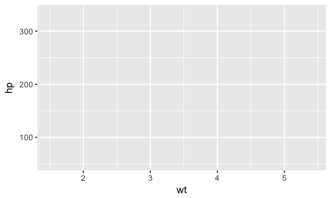

Now we can add geometric elements that take two inputs (x and y), like scatter:

my_plot +
  geom_point()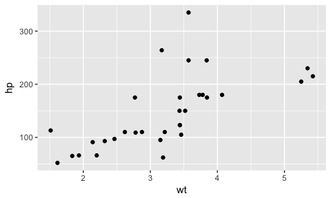

Or, maybe, a line:

my_plot +
  geom_line()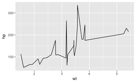

Or, perhaps a smoothed line with a confidence interval:

my_plot +
  geom_smooth()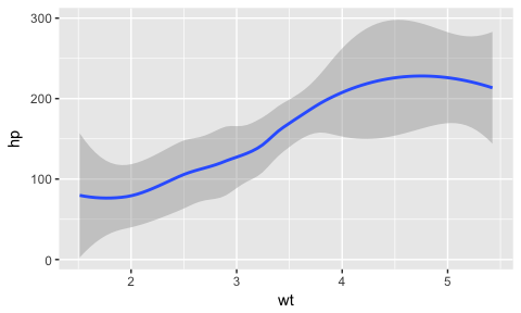

For now, let’s stick with a scatter plot. We can also add thematic elements like titles, colors, etc.:

my_fancy_plot <- ggplot(mtcars, aes(x=wt, y=hp)) +
  geom_point() +
  labs(title = "Horsepower as a function of weight",
       x = "Weight (in thousands of pounds)",
       y = "Horsepower") +
  theme(plot.background = element_rect(fill="light blue"))
my_fancy_plot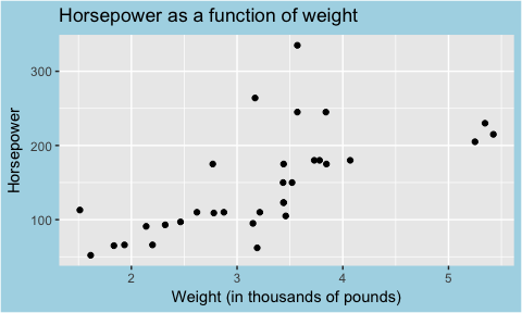

We can also use ggthemes to get pre-made styles that follow various popular formats, like the one used in The Economist magazine:

library(ggthemes)
my_economist_plot <- ggplot(mtcars, aes(x=wt, y=hp)) +
  geom_point() +
  labs(title = "Horsepower as a function of weight",
       x = "Weight (in thousands of pounds)",
       y = "Horsepower") +
  theme_economist_white()
my_economist_plot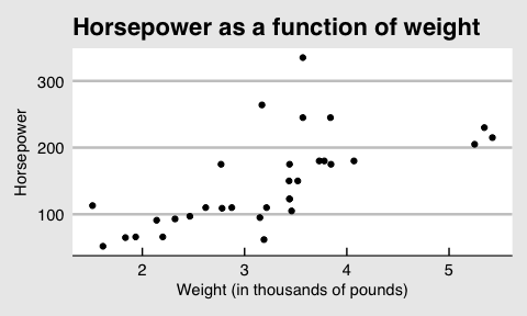

Within a geom, there are ways to change the particular implementation of that geometric element (point, bar, box…):

library(ggthemes)
my_economist_plot_2 <- ggplot(mtcars, aes(x=wt, y=hp)) +
  geom_point(color="red") +
  labs(title = "Horsepower as a function of weight",
       x = "Weight (in thousands of pounds)",
       y = "Horsepower") +
  theme_economist_white()
my_economist_plot_2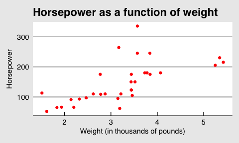

You get the idea.

Throw in a third variable, or more!

Ok, so now let’s get to the fun stuff. What if you wanted to show several scatter plots, according to number of cylinders? To do this, we’ll use “faceting”.

faceted_plot <- ggplot(mtcars, aes(wt, hp)) +
  geom_point() +
  facet_grid(. ~ cyl)
faceted_plot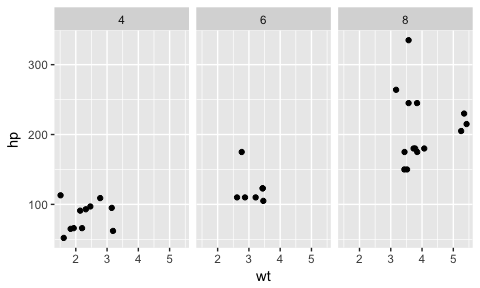

What if you don’t like that, but would like to see cylinder number as different point shapes in a single scatterplot?

shape_plot_1 <- ggplot(mtcars, aes(wt, hp)) +
  geom_point(aes(shape=as.factor(cyl)))
shape_plot_1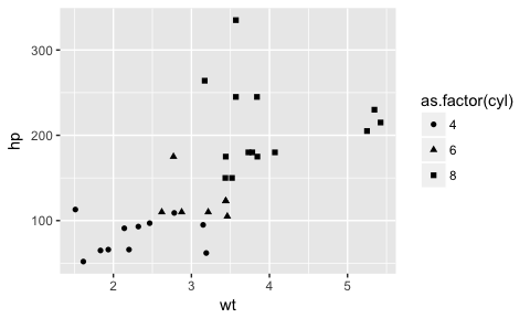

Let’s make it a little clearer with better labels, some colors, etc.:

shape_plot_2 <- ggplot(mtcars, aes(wt, hp)) +
  geom_point(aes(shape=as.factor(cyl), color = as.factor(cyl)),
             size = 3) + 
  theme_fivethirtyeight() +
    labs(title = "Horsepower as a function of weight") +
  theme_fivethirtyeight() +
  guides(color=guide_legend(title="Number of Cylinders")) +
  guides(shape=guide_legend(title="Number of Cylinders"))

shape_plot_2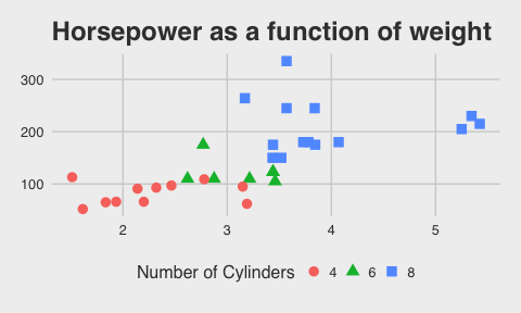

What if we wanted to make the size of the point based on the mpg? And, because there is some overlap between points, make the points somewhat transparent? Also, let’s change the theme.

shape_plot_3 <- ggplot(mtcars, aes(wt, hp)) +
  geom_point(aes(shape=as.factor(cyl), color = as.factor(cyl),
                 size = mpg), alpha = 0.7) + 
  theme_solarized() +
  labs(title = "Horsepower as a function of weight",
       x = "Weight (in thousands of pounds)",
       y = "Horsepower") +
  guides(color=guide_legend(title="Number of Cylinders")) +
  guides(shape=guide_legend(title="Number of Cylinders")) +
  guides(size=guide_legend(title="MPG"))
shape_plot_3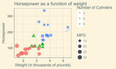

Other Plot types

Let’s take a look at other graphs, using various combinations of variables, with additional fun stuff thrown in.

density_plot_1 <- ggplot(mtcars, aes(qsec)) +
  geom_density() +
    labs(title = "Distribution of Quarter Mile Time",
       x = "Quarter Mile Time",
       y = "Probability Density")
density_plot_1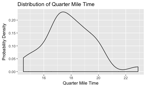

density_plot_2 <- ggplot(mtcars, aes(x = qsec, fill=as.factor(cyl))) +
  geom_density(alpha=0.4) +
    labs(title = "Distribution of Quarter Mile Time",
       x = "Quarter Mile Time",
       y = "Probability Density") +
  guides(fill=guide_legend(title="Number of\nCylinders\n"))
density_plot_2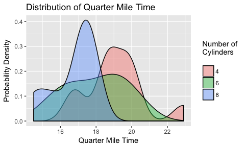

box_plot_1 <- ggplot(mtcars, aes(x=1, y = drat)) +
  geom_boxplot() +
  labs(y = "Rear Axle Ratio") +
  theme(axis.title.x=element_blank(),
        axis.text.x=element_blank(),
        axis.ticks.x=element_blank())
box_plot_1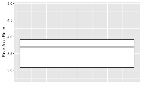

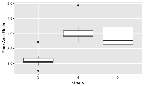
box_plot_2 <- ggplot(mtcars, aes(x=as.factor(gear), y = drat)) +
  geom_boxplot() +
  labs(x = "Gears", y = "Rear Axle Ratio") 
box_plot_2