Do Patterns in Missing Data Matter?
Yes. Yes they do.
Why Consider Something that isn’t There?
Our focus on missing data is typically on finding a way to eliminate it: replace it, ignore it, or just look sadly at it thinking what a lousy data set you have. Missing data can have value, however, especially if we can find patterns in it. You can’t find measures of central tendency like the mean or measures of dispersion like the variance and standard deviation in something that isn’t there, so how do you find whatever meaning your set of missing data carries and use that information to improve your study?
The Data
Our data set comes from Denmark, which has a Mycoplasma pneumoniae (M. pneumoniae) epidemic every 4 to 7 years. In 2016 Mia Søndergaard, et al. gathered data from the 2010 – 2011 epidemic, using medical records of various types, including diagnosis information, provider notes, and radiology records, for children younger than 16. They made their data public under a creative commons attribution license in 2018. Per the creative commons license, we provide a well-deserved citation: Søndergaard, Mia Johanna; Friis, Martin Barfred; Schrøder Hansen, Dennis; Jørgensen, Inger Merete (2018): Clinical manifestations in infants and children with Mycoplasma pneumoniae infection. PLOS ONE. Dataset.
Load the Data
We begin by loading the data into a data frame, then having a look at the variable names and dimensions. The shhh, shh, and sh functions are my own: I use them to suppress various warnings for the purpose of publication here. When you load your libraries, you might want to let them be noisy. The information in the various messages and warnings can be helpful.
shhh(shh(sh(library(tidyverse))))
shhh(shh(sh(library(readxl))))

# I did a little work on this data set to clean it before using it here.
pname <- "S1Dataset cleaned.xlsx"
# Load the data from a file
df <- read_excel(pname)

# Check it out
names(df)
##  [1] "ID"
##  [2] "Viral_Analysis_Number"
##  [3] "Virus"
##  [4] "Age"
##  [5] "Virus_YN"
##  [6] "Gender"
##  [7] "Weight_kg"
##  [8] "Height_cm"
##  [9] "Days_Admittd"
## [10] "Days_Since_First_Symptoms"
## [11] "Department"
## [12] "Exposed"
## [13] "Days_Since_Exposure"
## [14] "Prior_Pneumonia"
## [15] "Treated_YN"
## [16] "Fever"
## [17] "Febrile_Days"
## [18] "Cough"
## [19] "Cough_Days"
## [20] "Wheezing"
## [21] "Catharalia"
## [22] "Dyspnoea"
## [23] "Sore_Throat"
## [24] "Laryngitis"
## [25] "Ear_Pain"
## [26] "Any_Rash"
## [27] "Mild_Erythema"
## [28] "Hives"
## [29] "Vesicular_Rash"
## [30] "Steven_Johnson"
## [31] "Other_Rash"
## [32] "Lumbar_Puncture"
## [33] "CNS_DX"
## [34] "Nausea"
## [35] "Vomiting"
## [36] "Arthralgias"
## [37] "Artheritis"
## [38] "Renal_Symptoms"
## [39] "Cardiac"
## [40] "Raynaud_Phenomenon"
## [41] "Other_Symptoms"
## [42] "Temperature"
## [43] "Systolic"
## [44] "Diastolic"
## [45] "Conjunctivitis"
## [46] "Adenitis"
## [47] "Pharyngitis"
## [48] "Otoscopic"
## [49] "St_Pulm"
## [50] "Other"
## [51] "Pulse"
## [52] "O2_Saturation"
## [53] "RF"
## [54] "Tachypnoea"
## [55] "Treatment"
## [56] "Otner treatment"
## [57] "Antiobiotics_b4_Treatment"
## [58] "Days of treatment"
## [59] "Treatment started days after admission"
## [60] "Readmitted"
## [61] "Readmission_Comment"
## [62] "Hemoglobin"
## [63] "Leucocytes"
## [64] "Neutrophils"
## [65] "Monocytes"
## [66] "Lymphocytes"
## [67] "Trombocytes"
## [68] "CRP"
## [69] "Creatinin"
## [70] "Sodium"
## [71] "XR"
## [72] "Hilary_Adenopathy"
## [73] "Empyema"
## [74] "Pleuraleffusion"
## [75] "Atelectasis"
## [76] "Nodular_Infiltration"
## [77] "Infiltration_Location"
## [78] "Other_Comments"
dimensions <- dim(df)
The data is comprised of 143 cases and 78 variables, the names of which you can see in the above list.
Describe Patterns of Missingness
The best way to make sure that a description of missing data is available to you and your audience is to use plots. A good function for getting a visual description of missingness is in the naniar package, which was made public in November 2018 by Nicholas Tierney et al. (you can find out more about it, and them, here).
shhh(shh(sh(library(naniar))))
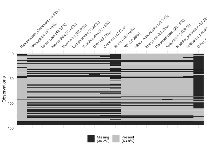
vis_miss(df)
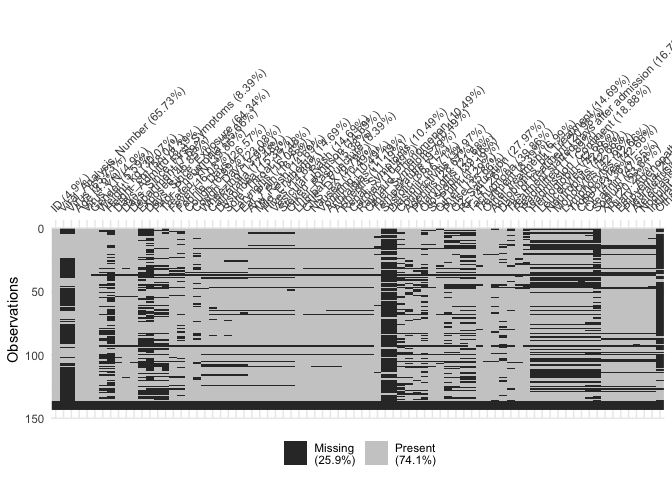
Okay, it’s a mess, because we have 78 variables that crowd the x axis, but the plot does tell us a few things: first, that there are some variables and variable groupings with very little data. That’s where there are thick black vertical lines. We might want to drop those variables once we figure out what they are. And at the bottom of the chart is a horizontal black line across all the varibles. Those are probably empty observations and we should get rid of them, too.
To get a better look, I used RStudio’s plot export function and saved the plot highly magnified. You might be able to get the same effect by running viz_miss(df) from the console and resizing the plot window until it takes up most of your screen. Then you can see which variables have a lot of missing values. Or we can do the easy thing and look at just some of the variables at a time instead of at the entire data set. Let’s do that.
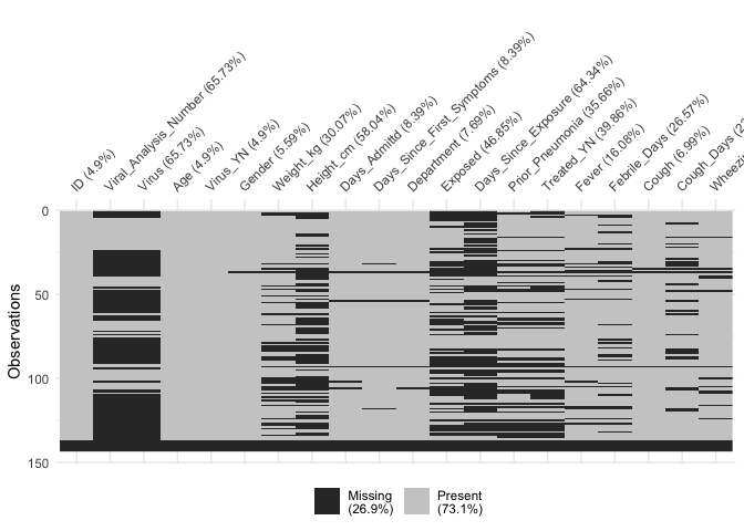
vis_miss(df[,1:20])
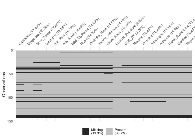
vis_miss(df[,21:40])
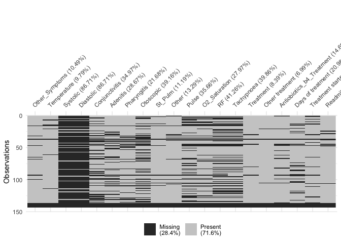
vis_miss(df[41:60])
vis_miss(df[61:78])
Let’s describe the interactions between missing values using another interesting package, UpSetR, which Alexander Lex (University of Utah), Nils Gehlenborg (Harvard Medical School), and Hendrik Strobelt, Romain Vuillemot, and Hanspeter Pfister
(all of Harvard University) created. Their work is fascinating, and you can find out more about it here. You can do a lot more with their package than what we’re doing here, but even this simple plot is very clever.
shhh(shh(sh(library(UpSetR))))
gg_miss_upset(df)
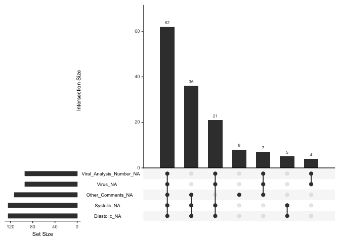
This plot shows a number of things. At the bottom right is a list of variables that gg_miss_upset() created to hold the missing values: around 90 observations are in the set Viral_Analysis_Number_NA or Virus_NA, which means they lack the variables on which those sets are based; around 110 are in the set Other_Comments_NA, and 120 are in the sets Systolic_NA and Diastolic_NA. Looking at the vertical bars, you can see that 62 cases lack all five of these variables, 36 lack the bottom three, and so on.
Why do these patterns matter? Looking at what isn’t there gives you information. Above we can see that there are some fairly logical patterns: virus analysis number and virus are always both missing; so are systolic and diastolic blood pressure. But suppose you have data in which people who work in certain jobs are less likely to report their income? Or what if a significant number of teenagers who leave unanswered a question about sexual preference also leave unanswered a question about suicidality? Unless you looked at the missing data you would not see potential peril to some of your study participants. Some information you can only find by examining missingness. As part of your initial survey of any data set, therefore, take a little extra time and look at the patterns of missingness.