
Comparing Parts of Speech with NLTK
In an earlier post, I showed you how to work with NLTK (the Natural Language Toolkit) in Python, using the texts that are optionally included with NLTK. There, we just sort of poked around trying various things. In this post, I will explain an actual statistical investigation of differences in the use of parts of speech using the same tools.
A bit of background: I recently ran a study comparing some parts of speech in blog posts by people who disclose an autism diagnosis to those parts of speech in blog posts by people without such a disclosure (presumed to not have autism). This is obviously messy public data not generated in a lab, but I found the signal I expected! You can view all the scripts used in my project at the GitHub repo for the study, if you’re interested.
In this post, we’re going to reproduce just the language analysis bit I used, not the web scraping. We’ll do the language analysis of parts of speech in State of the Union (SOTU) addresses. My (completely made up) hypothesis is that republicans and democrats differ in their use of comparative and superlative adjectives and adverbs (“best”, “most”, “angrier”, “grander”). I propose that one party has more extreme ways of describing the state of the nation in their State of the Union addresses.
Want to download this code instead of typing it yourself or copy/pasting? You can download:
- A Jupyter notebook of the code (recommended) or
- A python script of the code
Get Started
We’ll start with the obvious:
import nltkThen we’ll import some texts to work with. If you haven’t already (or, if it’s been awhile), do the following, and (in a new window), choose to download “all”. It might take a while, but it’s worth it to have a lot of texts and tools to play with:
nltk.download()Once that is accomplished (close the pop-up window), we can access some texts:
from nltk.corpus import state_unionLet’s take a peek at what’s inside!
state_union.fileids() ['1945-Truman.txt',
'1946-Truman.txt',
'1947-Truman.txt',
'1948-Truman.txt',
'1949-Truman.txt',
'1950-Truman.txt',
'1951-Truman.txt',
'1953-Eisenhower.txt',
'1954-Eisenhower.txt',
'1955-Eisenhower.txt',
'1956-Eisenhower.txt',
'1957-Eisenhower.txt',
'1958-Eisenhower.txt',
'1959-Eisenhower.txt',
'1960-Eisenhower.txt',
'1961-Kennedy.txt',
'1962-Kennedy.txt',
'1963-Johnson.txt',
'1963-Kennedy.txt',
'1964-Johnson.txt',
'1965-Johnson-1.txt',
'1965-Johnson-2.txt',
'1966-Johnson.txt',
'1967-Johnson.txt',
'1968-Johnson.txt',
'1969-Johnson.txt',
'1970-Nixon.txt',
'1971-Nixon.txt',
'1972-Nixon.txt',
'1973-Nixon.txt',
'1974-Nixon.txt',
'1975-Ford.txt',
'1976-Ford.txt',
'1977-Ford.txt',
'1978-Carter.txt',
'1979-Carter.txt',
'1980-Carter.txt',
'1981-Reagan.txt',
'1982-Reagan.txt',
'1983-Reagan.txt',
'1984-Reagan.txt',
'1985-Reagan.txt',
'1986-Reagan.txt',
'1987-Reagan.txt',
'1988-Reagan.txt',
'1989-Bush.txt',
'1990-Bush.txt',
'1991-Bush-1.txt',
'1991-Bush-2.txt',
'1992-Bush.txt',
'1993-Clinton.txt',
'1994-Clinton.txt',
'1995-Clinton.txt',
'1996-Clinton.txt',
'1997-Clinton.txt',
'1998-Clinton.txt',
'1999-Clinton.txt',
'2000-Clinton.txt',
'2001-GWBush-1.txt',
'2001-GWBush-2.txt',
'2002-GWBush.txt',
'2003-GWBush.txt',
'2004-GWBush.txt',
'2005-GWBush.txt',
'2006-GWBush.txt']
Well, our dataset is limited, but it’s good enough for us to get started!
We can peer inside one more carefully (here, I’m only showing a bit of the output):
print(state_union.raw('2006-GWBush.txt')) PRESIDENT GEORGE W. BUSH'S ADDRESS BEFORE A JOINT SESSION OF THE
CONGRESS ON THE STATE OF THE UNION
January 31, 2006
THE PRESIDENT: Thank you all. Mr. Speaker, Vice President Cheney,
members of Congress, members of the Supreme Court and diplomatic corps,
distinguished guests, and fellow citizens: Today our nation lost a
beloved, graceful, courageous woman who called America to its founding
ideals and carried on a noble dream. Tonight we are comforted by the
hope of a glad reunion with the husband who was taken so long ago, and
we are grateful for the good life of Coretta Scott King. (Applause.)...
Proof of Concept
First, we’ll create a function that will take a single text, and analyze it for parts of speech. First we’ll import a couple of needed modules:
from collections import Counter
from nltk.text import Text
And then we’ll create a function that turns the text to lower case, breaks it into words (tokenizing it), then assigns a part of speech for each token and returns the count for each part of speech in a dictionary:
def analyzeTextForPOS (text):
    # Tokenize the text
    tokens = nltk.word_tokenize(text.lower())
    text = nltk.Text(tokens)
    # get parts of speech for each token
    tags = nltk.pos_tag(text)
    # count how many times each pos is used
    counts = Counter(tag for word,tag in tags)
    # note that the POS abbreviations can be understood here:
    # https://www.ling.upenn.edu/courses/Fall_2003/ling001/penn_treebank_pos.html
    # return the counts as a dictionary
    return(dict(counts))
Let’s try the function to see if we get the kind of output we expect:
analyzeTextForPOS(state_union.raw('2006-GWBush.txt')) {'NN': 1080,
'VBD': 44,
'POS': 13,
'IN': 725,
'DT': 525,
'JJ': 515,
'CD': 71,
',': 319,
':': 81,
'PRP': 218,
'.': 336,
'NNS': 422,
'CC': 300,
'PRP$': 156,
'VBN': 110,
'WP': 19,
'TO': 175,
'VBP': 196,
'RB': 177,
'(': 68,
')': 68,
'VB': 328,
'RP': 17,
'RBS': 4,
'VBZ': 130,
'EX': 9,
'MD': 122,
'JJR': 44,
'WDT': 29,
'VBG': 121,
'PDT': 5,
'WRB': 9,
'RBR': 8,
'``': 1,
"''": 1,
'JJS': 7,
'$': 4}
The output is a bit confusing. We can go to the Penn Treebank homepage to find out what these labels mean. Or, we could do the following, which shows examples (output truncated for this post):
nltk.help.upenn_tagset() $: dollar
$ -$ --$ A$ C$ HK$ M$ NZ$ S$ U.S.$ US$
'': closing quotation mark
' ''
(: opening parenthesis
( [ {
): closing parenthesis
) ] }
,: comma
,
--: dash
--
.: sentence terminator
. ! ?
:: colon or ellipsis
: ; ...
CC: conjunction, coordinating
& 'n and both but either et for less minus neither nor or plus so
therefore times v. versus vs. whether yet
CD: numeral, cardinal
mid-1890 nine-thirty forty-two one-tenth ten million 0.5 one forty-
seven 1987 twenty '79 zero two 78-degrees eighty-four IX '60s .025
fifteen 271,124 dozen quintillion DM2,000 ...
DT: determiner
all an another any both del each either every half la many much nary
neither no some such that the them these this those
EX: existential there
there
FW: foreign word
gemeinschaft hund ich jeux habeas Haementeria Herr K'ang-si vous
lutihaw alai je jour objets salutaris fille quibusdam pas trop Monte
terram fiche oui corporis ...
Looking there, we discover, for example, that PRP is the label for personal pronoun (like me, you, they) and PRP$ is the label for possessive pronoun (like my, your, their).
Great, but how can we do this for every text, combining where needed (e.g. combining all of a single president’s SOTU addresses into one measurement) and comparing where appropriate (Republican vs Democrat, 1960s vs 1980s)? One approach is to build a table of counts such that we have all the counts for all the texts, and then we can remix as needed for our study.
Note that when we get into analysis like this, there are usually several ways to proceed – so if you would approach the problem differently, that’s okay!
Textual Analysis
We’re going to create a function that sets a few things up, then iterates over every file in the state of the union corpus and collects three sets of data:
- The “basic” data of the president’s name, the year of the address, and a sequence number, if applicable
- The “part of speech” data that counts each part of speech in that state of the union address
- The total parts of speech that were tagged
We’ll then combine these three sets into one single data frame, which we return as the result.
First, we need to load a couple of libraries:
import pandas as pd
import re
And now we’ll create the function that does all the good stuff!
def analyzeTexts():

    # Create a pattern for the regular expression (regex)
    # we're going to do further on.

    pattern = "(\d+)\-([A-Za-z]+)\-?(\d?)\.txt"
    # This pattern captures the date:     (\d+)
    # Then looks for a dash:              \-
    # Then captures a name:               ([A-Za-z]+)
    # Then looks for an optional dash:    \-?
    # Then captures an optional number:   (\d?)
    # Then looks for the .txt ending:     \.txt

    all_basic_info = []  # list of basic info dicts
    all_pos_info = []    # list of part of speech dicts
    all_totals = []      # list of total POS counted dicts

    # Note: we create three lists so that when we assemble
    # a data frame, these three types of information can be
    # placed in order, with basic info followed by pos counts
    # followed by total.  Since dicts are inherently unordered,
    # if we did a single list, we'd end up with columns in
    # alphabetical order, which is not what we want.


    # iterate over files and extract and organize data

    for filename in state_union.fileids():
        address_details = {}    # empty dict
        pos = {}                # empty dict
        totals = {}             # empty dict

        # Below, we're going to use  regular expressions to
        # extract meaningful info from the file name.

        m = re.match(pattern, filename)
        if m:
            address_details['address_date'] = m.group(1)
            address_details['president_name'] = m.group(2)
            address_details['optional_sequence'] = m.group(3)
            all_basic_info.append(address_details)  # add details of this file

            pos = analyzeTextForPOS(state_union.raw(filename))
            all_pos_info.append(pos)                # add part of speech for this file

            totals['Total'] = sum(pos.values())
            all_totals.append(totals)               # add total POS for this file

        else:
            print("Wonky problem with filename " + filename)

    return(pd.DataFrame(all_basic_info).join(pd.DataFrame(all_pos_info).join(pd.DataFrame(all_totals))))
    # return the results in a data frame -- leftmost columns are basic info,
    # then the part of speech info, then the totals in the rightmost column.
Now, let’s execute that function!
sotu_data = analyzeTexts()Take a peek at what we’ve built:
sotu_data| address_date | optional_sequence | president_name | $ | '' | ( | ) | , | . | : | ... | VBG | VBN | VBP | VBZ | WDT | WP | WP$ | WRB | `` | Total | |
|---|---|---|---|---|---|---|---|---|---|---|---|---|---|---|---|---|---|---|---|---|---|
| 0 | 1945 | Truman | NaN | 2.0 | NaN | NaN | 92 | 114 | 6 | ... | 24 | 55 | 46 | 38 | 8 | 6 | NaN | 4 | NaN | 2108 | |
| 1 | 1946 | Truman | 6.0 | 14.0 | 50.0 | 50.0 | 1026 | 1132 | 136 | ... | 391 | 938 | 596 | 537 | 210 | 45 | 2.0 | 48 | 17.0 | 29919 | |
| 2 | 1947 | Truman | NaN | 4.0 | 1.0 | 1.0 | 238 | 282 | 16 | ... | 97 | 165 | 162 | 113 | 40 | 11 | 1.0 | 17 | 4.0 | 6612 | |
| 3 | 1948 | Truman | 13.0 | NaN | NaN | NaN | 156 | 269 | 10 | ... | 88 | 133 | 151 | 99 | 41 | 8 | 2.0 | 14 | NaN | 5609 | |
| 4 | 1949 | Truman | 3.0 | 2.0 | NaN | NaN | 148 | 184 | 6 | ... | 57 | 91 | 105 | 72 | 29 | 3 | NaN | 2 | 2.0 | 3769 | |
| 5 | 1950 | Truman | 4.0 | NaN | NaN | NaN | 201 | 231 | 13 | ... | 78 | 133 | 166 | 113 | 40 | 12 | 1.0 | 6 | NaN | 5609 | |
| 6 | 1951 | Truman | 1.0 | 1.0 | NaN | NaN | 174 | 243 | 3 | ... | 70 | 69 | 165 | 76 | 23 | 10 | NaN | 6 | 1.0 | 4450 | |
| 7 | 1953 | Eisenhower | NaN | NaN | 12.0 | 12.0 | 286 | 339 | 65 | ... | 100 | 191 | 143 | 176 | 46 | 7 | 2.0 | 7 | NaN | 7706 | |
| 8 | 1954 | Eisenhower | 4.0 | NaN | 6.0 | 6.0 | 261 | 287 | 50 | ... | 92 | 163 | 145 | 131 | 38 | 11 | 3.0 | 18 | NaN | 6648 | |
| 9 | 1955 | Eisenhower | 4.0 | 3.0 | NaN | NaN | 369 | 331 | 65 | ... | 139 | 165 | 150 | 120 | 25 | 9 | 1.0 | 5 | 3.0 | 8086 | |
| 10 | 1956 | Eisenhower | NaN | NaN | NaN | NaN | 333 | 371 | 62 | ... | 127 | 273 | 170 | 158 | 44 | 8 | 3.0 | 10 | NaN | 9051 | |
| 11 | 1957 | Eisenhower | NaN | NaN | 4.0 | 4.0 | 178 | 187 | 39 | ... | 56 | 105 | 103 | 97 | 37 | 8 | 2.0 | 4 | NaN | 4587 | |
| 12 | 1958 | Eisenhower | 3.0 | 5.0 | NaN | NaN | 258 | 246 | 41 | ... | 85 | 93 | 120 | 132 | 38 | 9 | NaN | 7 | 6.0 | 5500 | |
| 13 | 1959 | Eisenhower | 3.0 | 1.0 | NaN | NaN | 196 | 261 | 38 | ... | 87 | 137 | 155 | 105 | 31 | 7 | 1.0 | 15 | 1.0 | 5550 | |
| 14 | 1960 | Eisenhower | 3.0 | 5.0 | NaN | NaN | 262 | 253 | 37 | ... | 98 | 141 | 136 | 144 | 49 | 6 | NaN | 7 | 5.0 | 6230 | |
| 15 | 1961 | Kennedy | NaN | 3.0 | NaN | NaN | 302 | 222 | 108 | ... | 89 | 160 | 180 | 134 | 44 | 20 | 1.0 | 20 | 2.0 | 6546 | |
| 16 | 1962 | Kennedy | 7.0 | 12.0 | NaN | NaN | 347 | 262 | 178 | ... | 104 | 155 | 149 | 154 | 28 | 12 | 6.0 | 10 | 12.0 | 7483 | |
| 17 | 1963 | Johnson | NaN | 2.0 | NaN | NaN | 93 | 72 | 28 | ... | 13 | 28 | 42 | 31 | 10 | 11 | NaN | 2 | 2.0 | 1857 | |
| 18 | 1963 | Kennedy | 12.0 | 4.0 | NaN | NaN | 301 | 220 | 90 | ... | 95 | 106 | 139 | 152 | 28 | 20 | 2.0 | 9 | 4.0 | 6132 | |
| 19 | 1964 | Johnson | 14.0 | 2.0 | NaN | NaN | 186 | 136 | 42 | ... | 57 | 49 | 45 | 39 | 20 | 10 | NaN | 6 | 2.0 | 3624 | |
| 20 | 1965 | 1 | Johnson | 2.0 | 3.0 | 1.0 | 1.0 | 124 | 259 | 63 | ... | 55 | 78 | 147 | 89 | 28 | 11 | 2.0 | 19 | 3.0 | 4922 |
| 21 | 1965 | 2 | Johnson | NaN | 8.0 | NaN | NaN | 165 | 196 | 41 | ... | 30 | 100 | 117 | 103 | 17 | 26 | 1.0 | 16 | 2.0 | 4188 |
| 22 | 1966 | Johnson | 19.0 | NaN | 1.0 | 1.0 | 246 | 260 | 73 | ... | 78 | 108 | 173 | 106 | 38 | 31 | 5.0 | 10 | NaN | 6194 | |
| 23 | 1967 | Johnson | 24.0 | 22.0 | NaN | NaN | 301 | 352 | 121 | ... | 111 | 176 | 239 | 140 | 37 | 22 | 2.0 | 29 | 20.0 | 8148 | |
| 24 | 1968 | Johnson | 35.0 | 1.0 | NaN | NaN | 192 | 252 | 144 | ... | 65 | 108 | 159 | 98 | 26 | 23 | NaN | 12 | 1.0 | 5597 | |
| 25 | 1969 | Johnson | 13.0 | 7.0 | NaN | NaN | 188 | 197 | 53 | ... | 53 | 141 | 177 | 97 | 27 | 11 | NaN | 11 | 5.0 | 4615 | |
| 26 | 1970 | Nixon | 6.0 | NaN | NaN | NaN | 230 | 205 | 8 | ... | 53 | 92 | 136 | 103 | 54 | 13 | 1.0 | 20 | NaN | 4982 | |
| 27 | 1971 | Nixon | 4.0 | NaN | NaN | NaN | 165 | 174 | 13 | ... | 59 | 77 | 93 | 70 | 38 | 25 | NaN | 20 | NaN | 4510 | |
| 28 | 1972 | Nixon | 1.0 | NaN | NaN | NaN | 217 | 174 | 31 | ... | 93 | 94 | 144 | 82 | 35 | 21 | NaN | 9 | NaN | 4471 | |
| 29 | 1973 | Nixon | NaN | NaN | NaN | NaN | 81 | 62 | 6 | ... | 33 | 34 | 46 | 25 | 18 | 1 | 2.0 | 6 | NaN | 1859 | |
| ... | ... | ... | ... | ... | ... | ... | ... | ... | ... | ... | ... | ... | ... | ... | ... | ... | ... | ... | ... | ... | ... |
| 35 | 1979 | Carter | 3.0 | 8.0 | NaN | NaN | 198 | 159 | 19 | ... | 46 | 80 | 97 | 67 | 24 | 9 | NaN | 7 | 8.0 | 3713 | |
| 36 | 1980 | Carter | NaN | 2.0 | NaN | NaN | 136 | 163 | 30 | ... | 42 | 78 | 83 | 65 | 26 | 3 | NaN | 6 | 2.0 | 3807 | |
| 37 | 1981 | Reagan | 27.0 | 3.0 | NaN | NaN | 214 | 218 | 31 | ... | 99 | 118 | 164 | 99 | 30 | 24 | NaN | 9 | 3.0 | 5041 | |
| 38 | 1982 | Reagan | 10.0 | 14.0 | NaN | NaN | 276 | 251 | 49 | ... | 83 | 120 | 161 | 81 | 28 | 30 | 1.0 | 21 | 14.0 | 5908 | |
| 39 | 1983 | Reagan | 4.0 | 5.0 | NaN | NaN | 321 | 252 | 48 | ... | 104 | 123 | 150 | 103 | 35 | 22 | NaN | 9 | 5.0 | 6302 | |
| 40 | 1984 | Reagan | 7.0 | 5.0 | NaN | NaN | 264 | 293 | 52 | ... | 100 | 106 | 141 | 127 | 21 | 20 | 1.0 | 21 | 5.0 | 5681 | |
| 41 | 1985 | Reagan | 4.0 | 4.0 | NaN | NaN | 238 | 222 | 44 | ... | 103 | 88 | 155 | 109 | 23 | 20 | 3.0 | 14 | 4.0 | 4834 | |
| 42 | 1986 | Reagan | 2.0 | 4.0 | NaN | NaN | 214 | 173 | 40 | ... | 69 | 55 | 107 | 81 | 18 | 10 | 2.0 | 15 | 4.0 | 4010 | |
| 43 | 1987 | Reagan | 4.0 | 17.0 | NaN | NaN | 198 | 202 | 46 | ... | 74 | 79 | 117 | 99 | 17 | 19 | 3.0 | 11 | 13.0 | 4389 | |
| 44 | 1988 | Reagan | 5.0 | 7.0 | 1.0 | 2.0 | 272 | 215 | 112 | ... | 91 | 96 | 135 | 141 | 38 | 31 | 2.0 | 20 | 7.0 | 5576 | |
| 45 | 1989 | Bush | 8.0 | 19.0 | NaN | NaN | 266 | 289 | 59 | ... | 72 | 103 | 175 | 92 | 25 | 21 | 2.0 | 11 | 20.0 | 5583 | |
| 46 | 1990 | Bush | 3.0 | 4.0 | NaN | NaN | 237 | 198 | 77 | ... | 45 | 59 | 127 | 128 | 24 | 18 | 1.0 | 24 | 4.0 | 4414 | |
| 47 | 1991 | 1 | Bush | 4.0 | 2.0 | NaN | NaN | 237 | 226 | 56 | ... | 58 | 73 | 136 | 124 | 21 | 21 | NaN | 23 | 2.0 | 4555 |
| 48 | 1991 | 2 | Bush | NaN | 4.0 | NaN | NaN | 150 | 182 | 32 | ... | 34 | 61 | 72 | 55 | 12 | 15 | 2.0 | 6 | 4.0 | 3292 |
| 49 | 1992 | Bush | 12.0 | 8.0 | NaN | NaN | 286 | 321 | 38 | ... | 72 | 83 | 206 | 133 | 41 | 46 | NaN | 18 | 8.0 | 5896 | |
| 50 | 1993 | Clinton | 19.0 | 2.0 | NaN | NaN | 340 | 289 | 30 | ... | 126 | 101 | 291 | 141 | 39 | 50 | NaN | 18 | 2.0 | 7809 | |
| 51 | 1994 | Clinton | 6.0 | 11.0 | NaN | NaN | 430 | 396 | 33 | ... | 119 | 105 | 307 | 138 | 35 | 81 | 5.0 | 40 | 10.0 | 8431 | |
| 52 | 1995 | Clinton | 14.0 | 9.0 | NaN | NaN | 469 | 457 | 47 | ... | 150 | 158 | 391 | 179 | 41 | 78 | 1.0 | 43 | 8.0 | 10415 | |
| 53 | 1996 | Clinton | 6.0 | 3.0 | NaN | NaN | 304 | 356 | 31 | ... | 122 | 101 | 285 | 136 | 31 | 41 | NaN | 21 | 2.0 | 7129 | |
| 54 | 1997 | Clinton | 6.0 | 3.0 | NaN | NaN | 389 | 338 | 44 | ... | 95 | 88 | 197 | 127 | 36 | 31 | 3.0 | 19 | 3.0 | 7634 | |
| 55 | 1998 | Clinton | 5.0 | 9.0 | NaN | NaN | 424 | 368 | 89 | ... | 124 | 109 | 304 | 130 | 44 | 30 | NaN | 33 | 9.0 | 8380 | |
| 56 | 1999 | Clinton | 12.0 | 14.0 | NaN | NaN | 460 | 385 | 59 | ... | 123 | 127 | 266 | 124 | 25 | 33 | NaN | 16 | 14.0 | 8578 | |
| 57 | 2000 | Clinton | 14.0 | 9.0 | NaN | NaN | 511 | 486 | 82 | ... | 168 | 139 | 371 | 164 | 54 | 49 | NaN | 29 | 8.0 | 10379 | |
| 58 | 2001 | 1 | GWBush | 17.0 | 2.0 | 94.0 | 94.0 | 221 | 378 | 30 | ... | 74 | 72 | 158 | 127 | 18 | 22 | NaN | 12 | 2.0 | 5369 |
| 59 | 2001 | 2 | GWBush | 1.0 | 1.0 | 31.0 | 31.0 | 187 | 211 | 58 | ... | 54 | 81 | 109 | 73 | 11 | 25 | NaN | 10 | 1.0 | 3577 |
| 60 | 2002 | GWBush | 1.0 | 4.0 | 77.0 | 77.0 | 218 | 283 | 70 | ... | 62 | 85 | 132 | 85 | 15 | 21 | 1.0 | 6 | 4.0 | 4701 | |
| 61 | 2003 | GWBush | NaN | 4.0 | NaN | NaN | 325 | 280 | 98 | ... | 104 | 132 | 168 | 149 | 29 | 20 | NaN | 14 | 4.0 | 6138 | |
| 62 | 2004 | GWBush | 7.0 | 5.0 | 72.0 | 72.0 | 342 | 347 | 50 | ... | 144 | 117 | 197 | 115 | 21 | 22 | NaN | 13 | 3.0 | 6211 | |
| 63 | 2005 | GWBush | 3.0 | 9.0 | 68.0 | 68.0 | 322 | 299 | 65 | ... | 95 | 101 | 163 | 123 | 40 | 15 | 1.0 | 16 | 7.0 | 6018 | |
| 64 | 2006 | GWBush | 4.0 | 1.0 | 68.0 | 68.0 | 319 | 336 | 81 | ... | 121 | 110 | 196 | 130 | 29 | 19 | NaN | 9 | 1.0 | 6457 |
Keep in mind that the numbers in the part of speech columns are just counts! We’ll have to figure out percentages, since we want to compare the relative frequency of parts of speech.
Also, we want to combine the part of speech counts and the total parts of speech counted for each president – so, all of Nixon’s SOTU speeches combined into one count, etc. The reason for this is that the number of speeches for each president are unbalanced. If we don’t combine them, we risk over-weighting the influence of one president compared to another in our statistical analysis.
We also have too many parts of speech to work with. We really want to work with just a handful.
So, we have to slim down and consolidate our large data frame. We can do this by indexing and by using the pandas groupby function.
We’ll do this in steps. First, we’ll get all rows and just the columns starting with president_name forward.
sotu_by_president = sotu_data.loc[:,'president_name':]Then we’ll aggregate (combine rows) by president name:
sotu_by_president = sotu_by_president.groupby('president_name').sum() Let’s take a peek so far:
sotu_by_president| $ | '' | ( | ) | , | . | : | CC | CD | DT | ... | VBG | VBN | VBP | VBZ | WDT | WP | WP$ | WRB | `` | Total | |
|---|---|---|---|---|---|---|---|---|---|---|---|---|---|---|---|---|---|---|---|---|---|
| president_name | |||||||||||||||||||||
| Bush | 27.0 | 37.0 | 0.0 | 0.0 | 1176 | 1216 | 262 | 1024 | 226 | 2257 | ... | 281 | 379 | 716 | 532 | 123 | 121 | 5.0 | 82 | 38.0 | 23740 |
| Carter | 13.0 | 11.0 | 0.0 | 0.0 | 580 | 571 | 53 | 600 | 130 | 1231 | ... | 138 | 252 | 337 | 233 | 80 | 34 | 1.0 | 34 | 11.0 | 12690 |
| Clinton | 82.0 | 60.0 | 0.0 | 0.0 | 3327 | 3075 | 415 | 2514 | 937 | 5932 | ... | 1027 | 928 | 2412 | 1139 | 305 | 393 | 9.0 | 219 | 56.0 | 68755 |
| Eisenhower | 17.0 | 14.0 | 22.0 | 22.0 | 2143 | 2275 | 397 | 1919 | 473 | 5399 | ... | 784 | 1268 | 1122 | 1063 | 308 | 65 | 12.0 | 73 | 15.0 | 53358 |
| Ford | 40.0 | 7.0 | 0.0 | 0.0 | 641 | 685 | 129 | 585 | 279 | 1432 | ... | 217 | 298 | 420 | 261 | 86 | 32 | 0.0 | 34 | 7.0 | 15462 |
| GWBush | 33.0 | 26.0 | 410.0 | 410.0 | 1934 | 2134 | 452 | 1699 | 423 | 3060 | ... | 654 | 698 | 1123 | 802 | 163 | 144 | 2.0 | 80 | 22.0 | 38471 |
| Johnson | 107.0 | 45.0 | 2.0 | 2.0 | 1495 | 1724 | 565 | 1662 | 576 | 3912 | ... | 462 | 788 | 1099 | 703 | 203 | 145 | 10.0 | 105 | 35.0 | 39145 |
| Kennedy | 19.0 | 19.0 | 0.0 | 0.0 | 950 | 704 | 376 | 982 | 250 | 1955 | ... | 288 | 421 | 468 | 440 | 100 | 52 | 9.0 | 39 | 18.0 | 20161 |
| Nixon | 17.0 | 0.0 | 0.0 | 0.0 | 953 | 817 | 66 | 710 | 302 | 2423 | ... | 336 | 432 | 573 | 392 | 203 | 81 | 3.0 | 67 | 0.0 | 21575 |
| Reagan | 63.0 | 59.0 | 1.0 | 2.0 | 1997 | 1826 | 422 | 1674 | 625 | 3692 | ... | 723 | 785 | 1130 | 840 | 210 | 176 | 12.0 | 120 | 55.0 | 41741 |
| Truman | 27.0 | 23.0 | 51.0 | 51.0 | 2035 | 2455 | 190 | 1983 | 1136 | 5997 | ... | 805 | 1584 | 1391 | 1048 | 391 | 95 | 6.0 | 97 | 24.0 | 58076 |
And we’ll limit to just comparative and superlative adjectives and adverbs. But we’ll also hang on to ‘Total’, because that allows us to determine the percentage of speech that each part of speech takes up.
cols_i_want = ['JJR', 'JJS','RBR','RBS', 'Total']
sotu_by_president = sotu_by_president.loc[:,cols_i_want]
We’ll separate out republicans from democrats:
republicans = ['Bush','Eisenhower','Ford','Nixon','Reagan','GWBush']
democrats = ['Carter','Clinton','Johnson','Kennedy','Truman']

republican_speech = sotu_by_president.loc[sotu_by_president.index.isin(republicans)]
democrat_speech = sotu_by_president.loc[sotu_by_president.index.isin(democrats)]
Let’s take a quick peek:
republican_speech| JJR | JJS | RBR | RBS | Total | |
|---|---|---|---|---|---|
| president_name | |||||
| Bush | 102 | 44 | 41 | 12.0 | 23740 |
| Eisenhower | 212 | 80 | 100 | 43.0 | 53358 |
| Ford | 96 | 42 | 46 | 12.0 | 15462 |
| GWBush | 210 | 72 | 55 | 22.0 | 38471 |
| Nixon | 116 | 49 | 62 | 23.0 | 21575 |
| Reagan | 215 | 98 | 79 | 29.0 | 41741 |
democrat_speech| JJR | JJS | RBR | RBS | Total | |
|---|---|---|---|---|---|
| president_name | |||||
| Carter | 65 | 26 | 21 | 9.0 | 12690 |
| Clinton | 457 | 230 | 166 | 55.0 | 68755 |
| Johnson | 206 | 105 | 64 | 30.0 | 39145 |
| Kennedy | 76 | 39 | 39 | 15.0 | 20161 |
| Truman | 217 | 99 | 67 | 35.0 | 58076 |
Now we have some nice, compact data frames! We still have to figure out percentages, however. We’ll divide everything by the ‘Total’ column:
democrat_speech = democrat_speech.div(democrat_speech['Total'], axis=0)
republican_speech = republican_speech.div(republican_speech['Total'], axis=0)
Statistical Analysis
Do Republicans and Democrats differ in the way they use comparative and superlative adjectives and adverbs in their State of the Union addresses? Let’s take each type of part of speech separately and compare them, then sum all four parts of speech and make an overall comparison as well. We’ll visualize differences using a box plot, and also conduct a two-sample T test.
We’ll need some additional python libraries, and need to set up some plot parameters to display our visualizations in our Jupyter Notebook:
from scipy.stats import ttest_ind
from statistics import mean, stdev
from math import sqrt
import matplotlib.pyplot as plt
%matplotlib inline
plt.rcParams.update({'font.size': 18})
And now we’ll plot the comparative adjective use of both groups.
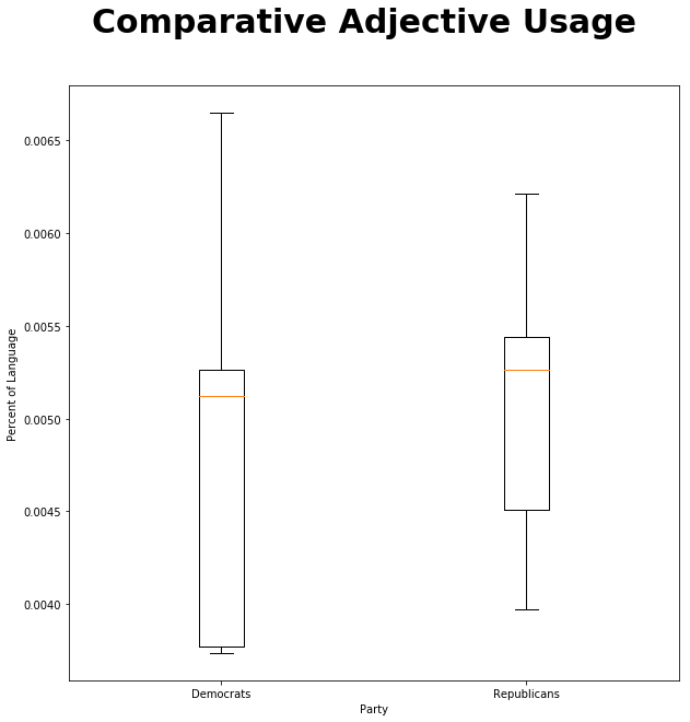
It doesn’t look very promising – these distributions overlap rather a lot! Let’s do a T test to see if the difference is likely due to random variation:
ttest_ind(republican_speech["JJR"],democrat_speech["JJR"]) Ttest_indResult(statistic=0.27734514630142165, pvalue=0.7877802746796846)
That’s a very high p value. 78.8% probability that the differences we see are due to random chance, not a true group difference.
Let’s move on to superlative adjectives!
fig = plt.figure(figsize=(10,10))
fig.suptitle('Superlative Adjective Usage', fontsize=30, fontweight='bold')

ax = fig.add_subplot(111)
ax.boxplot([democrat_speech["JJS"],republican_speech["JJS"]], labels=["Democrats", "Republicans"])

ax.set_xlabel('Party')
ax.set_ylabel('Percent of Language')

plt.show()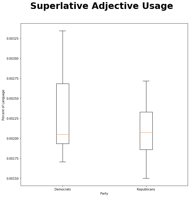
ttest_ind(republican_speech["JJS"],democrat_speech["JJS"]) Ttest_indResult(statistic=-0.7498826364182734, pvalue=0.47247171059893134)
Once again, both visually and statistically, there’s no significant difference. Let’s do the same for both comparative and superlative adjectives!
fig = plt.figure(figsize=(10,10))
fig.suptitle('Comparative Adverb Usage', fontsize=30, fontweight='bold')

ax = fig.add_subplot(111)
ax.boxplot([democrat_speech["RBR"],republican_speech["RBR"]], labels=["Democrats", "Republicans"])

ax.set_xlabel('Party')
ax.set_ylabel('Percent of Language')

plt.show()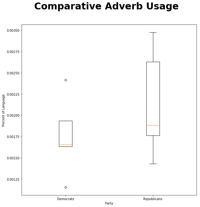
ttest_ind(republican_speech["JJS"],democrat_speech["JJS"]) Ttest_indResult(statistic=1.0781202441947808, pvalue=0.30902662581074575)
fig = plt.figure(figsize=(10,10))
fig.suptitle('Superlative Adverb Usage', fontsize=30, fontweight='bold')

ax = fig.add_subplot(111)
ax.boxplot([democrat_speech["RBS"],republican_speech["RBS"]], labels=["Democrats", "Republicans"])

ax.set_xlabel('Party')
ax.set_ylabel('Percent of Language')

plt.show()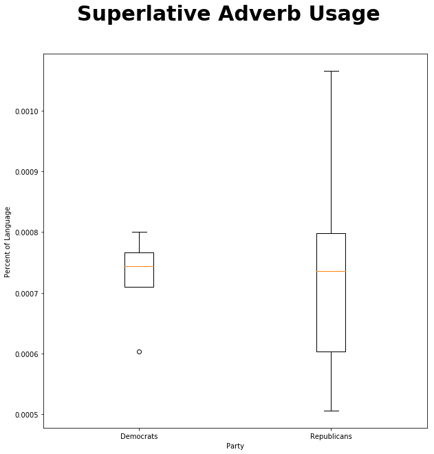
ttest_ind(republican_speech["RBS"],democrat_speech["RBS"]) Ttest_indResult(statistic=0.12929601859348358, pvalue=0.8999668706431508)
Well, none of the individual parts of speech were notably different, but what if we sum them?
republican_all = republican_speech["JJR"] + republican_speech["JJS"] + republican_speech["RBR"] + republican_speech["RBS"]
democrat_all = democrat_speech["JJR"] + democrat_speech["JJS"] + democrat_speech["RBR"] + democrat_speech["RBS"]

ttest_ind(republican_all,democrat_all)
Ttest_indResult(statistic=0.2468003972480926, pvalue=0.8106000875259137)
Nope, no finding here. It looks like we can reject my hypothesis that presidential speakers of different parties express different concentrations of comparative and superlative adjectives and adverbs!
How could this investigation have been done better? Well, we’d ideally like more text from more presidents – maybe get all of the SOTU addresses instead of a small chunk of years, or add in other texts. We also want to be careful to remove annotations like “(Applause)” and photo credits, which aren’t really part of the presidential address. We didn’t do that here. There are lots of ways to remix this. Let me know what you come up with and if you use this technique in your research!