
Linear Algebra, a Geometric Approach
Linear algebra is unfortunately often taught arithmetically, with rote memorization of how to work with vectors and matrices. A semester, or a year, or a decade goes by, and the core concepts of linear algebra tend to be forgotten in a way that basic algebra, geometry, and even calculus are not. If it’s been a few years since you’ve used calculus, you probably can’t spontaneously get the derivative of f(x) = sin(x) + 2x + 5, but you understand what a derivative is and why it’s important. Concepts like rate of change, tangent line, slope, and area under a curve are fairly easily retained, even when specific formulas are not. Linear algebra, in my experience, doesn’t stick in the same way.
Linear algebra is important in research, where we have several variables (dimensions) that describe observations, and we have predictions or comparisons to make in that multi-dimensional reality. Linear algebra, at its core, is the study of answering questions about multi-dimensional “space” and an extension of the math we intuitively perform in 2 and 3 dimensions.
In 2-dimensional space, we may do something like map weight as a function of height, so that height is represented by the x-axis, and weight on the y-axis. We intuitively know how to find the distance between two points in this space – we use the Pythagorean theorem to figure it out. If we imagined that we have the true height and weight of a given elephant plotted as a dot on the cartesian plane, and we had various guesses about its height and weight plotted as well, we could easily figure out which guess was the closest by measuring distance – squaring the difference between the true and guessed height, and squaring it, adding the squared difference between the true and guessed weight (maybe counting in thousands of kg), and taking the square root.
{:}
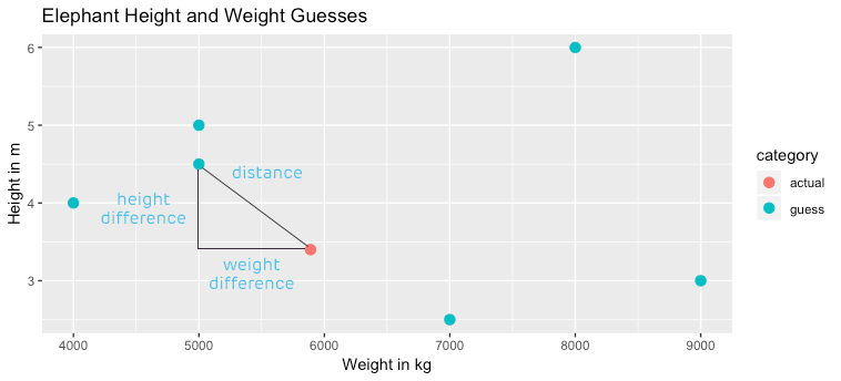
Does this sound familiar? When we measure the root mean square error of a linear model, we take the distance between actual and predicted points (the residuals), square them all, average those squared values for normalization, and take the square root. It’s similar to the Pythagorean theorem, which makes sense, because RMSE is a measure of distance – the distance between our prediction and observed reality. Yet, RMSE is seldom described geometrically or as a distance metric, and we often hear and read descriptions of the calculation with words like “we square the residuals to make them positive”. While it’s true that squaring residuals makes them positive, that’s not why we square them. We square them because we want to find distance.
Also, when we think about dimension reduction in a highly dimensional dataset (lots of columns), it helps to think geometrically and understand the “angle” between each variable. Consider, for example, the Etch A Sketch, a toy with two dials that allows you to draw. One dial goes left and right only. If you only had that dial, you’d be able to get to any point in that left-right line, but nothing else. Luckily, there’s a second dial that moves in a line that’s 90° distant from the left-right dial. It’s the up-down dial. With those two dials together, you can draw anything in the plane. That second dial is extremely useful because it’s perpendicular to the first. If it weren’t perpendicular (say, it drew at a 45° angle) you’d still be able to draw anything in 2 dimensions, but it would be more work, because when you used the second dial, you’d always be dividing your efforts equally between moving up/down and right/left. Perpendicular angles are the simplest solution to drawing in 2 dimensions.
Video just for fun, and to demonstrate that with two perpendicular vectors you can access (span) the entire plane.
When we extend the Etch A Sketch model a bit, we consider what we’d have to add to get our Etch A Sketch to draw in 3 dimensions. We’d need a third dial that would send a line directly through the center of the Etch A Sketch, which was at 90° to both of the other dials (a sort of z-axis, if you will). Four or more dimensions boggles our 3D minds, but we have a linear algebra term for getting the most useful “dials” – orthogonality. When we reduce multi-dimensional data down, we want to get the most un-combined “dials” possible – it’s better to get a dial that does something brand new rather than a dial that adds something new but kind of runs at a 45° angle, repeating the effort of another dial. The task of recombining variables to come up with the best set of variables that are correlated to each other as little as possible is called Principle Components Analysis, or PCA.
Understanding linear algebra geometrically can help you understand statistical concepts and measures that rely on linear algebra, and allow you to have some instinct about linear algebra, even if you don’t know how to calculate the determinant of a matrix or give the formal definition of an eigenvector. If you liked this article and the geometric intuitions I tried to impart, I highly recommend you check out the “Essence of Linear Algebra” series published by 3Blue1Brown. This author’s methods of explaining complex linear algebra concepts in a visually delightful and easy-to-understand way are unmatched.