
Intro to NetworkX
After reading below, download the jupyter notebook (here, my work was in Python 3) that contains the code and descriptions in this article. Want just the python, without the notebook? Use this link instead!
NetworkX Example
networkx is a python module that allows you to build networks (or graphs). This can come in handy in linking data points by similarity, by genetic relationship, by proximity, etc. Networks can be useful in finding patterns in data and visualizing data clusters. Networks consist of nodes that are connected by edges. Both nodes and edges can have associated details. Consider, for example, a food poisoning graph, where individuals and food suppliers are nodes, and edges are the “ate food from” relationship. Node details could include age and sex, while edge details could include approximate time of food consumption or type of food consumed.
In this tutorial, we’ll take a simple, prebuilt network and analyze it. You may need to install networkx using pip or conda.
Step 1: Load packages and data
The Davis dataset was collected by Davis et al. in the 1930s. Data represent observed attendance at 14 social events by 18 Southern women. The graph is bipartite (events, women). We’ll plot our networks using inline (i.e. in-the-notebook) matplotlib.
import networkx as nx
import networkx.algorithms.bipartite as bipartite

import matplotlib.pyplot as plt
%matplotlib inline

import pandas as pd

G = nx.davis_southern_women_graph()
Step 2: Investigate network nodes
Let’s take a look at the nodes in our graph:
G.nodes(data = True)NodeDataView({'Evelyn Jefferson': {'bipartite': 0}, 'Laura Mandeville':
{'bipartite': 0}, 'Theresa Anderson': {'bipartite': 0}, 'Brenda
Rogers': {'bipartite': 0}, 'Charlotte McDowd': {'bipartite': 0},
'Frances Anderson': {'bipartite': 0}, 'Eleanor Nye': {'bipartite': 0},
'Pearl Oglethorpe': {'bipartite': 0}, 'Ruth DeSand': {'bipartite': 0},
'Verne Sanderson': {'bipartite': 0}, 'Myra Liddel': {'bipartite': 0},
'Katherina Rogers': {'bipartite': 0}, 'Sylvia Avondale': {'bipartite':
0}, 'Nora Fayette': {'bipartite': 0}, 'Helen Lloyd': {'bipartite': 0},
'Dorothy Murchison': {'bipartite': 0}, 'Olivia Carleton': {'bipartite':
0}, 'Flora Price': {'bipartite': 0}, 'E1': {'bipartite': 1}, 'E2':
{'bipartite': 1}, 'E3': {'bipartite': 1}, 'E4': {'bipartite': 1}, 'E5':
{'bipartite': 1}, 'E6': {'bipartite': 1}, 'E7': {'bipartite': 1}, 'E8':
{'bipartite': 1}, 'E9': {'bipartite': 1}, 'E10': {'bipartite': 1},
'E11': {'bipartite': 1}, 'E12': {'bipartite': 1}, 'E13': {'bipartite':
1}, 'E14': {'bipartite': 1}})
This looks like a bipartite set, from looking at the details associated with each node. Let’s see if it’s set up that way!
print (bipartite.sets(G))({'Evelyn Jefferson', 'Verne Sanderson', 'Eleanor Nye', 'Katherina
Rogers', 'Nora Fayette', 'Ruth DeSand', 'Myra Liddel', 'Laura
Mandeville', 'Pearl Oglethorpe', 'Flora Price', 'Charlotte McDowd',
'Frances Anderson', 'Brenda Rogers', 'Dorothy Murchison', 'Helen Lloyd',
'Olivia Carleton', 'Theresa Anderson', 'Sylvia Avondale'}, {'E3', 'E5',
'E11', 'E1', 'E6', 'E2', 'E14', 'E9', 'E7', 'E10', 'E12', 'E13', 'E8',
'E4'})
We have two kinds of nodes: women, and events, in that order. Let’s assign the nodes to corresponding variables so that we can look at women and events separately. For example, we may want to understand how closely socially linked the women are to each other.
women, events = bipartite.sets(G)
print ("\nWomen:\n" + str(list(women)))
print ("\nEvents:\n" + str(list(events)))
Women:
['Evelyn Jefferson', 'Verne Sanderson', 'Eleanor Nye', 'Katherina
Rogers', 'Nora Fayette', 'Ruth DeSand', 'Myra Liddel', 'Laura
Mandeville', 'Pearl Oglethorpe', 'Flora Price', 'Charlotte McDowd',
'Frances Anderson', 'Brenda Rogers', 'Dorothy Murchison', 'Helen Lloyd',
'Olivia Carleton', 'Theresa Anderson', 'Sylvia Avondale']
Events:
['E3', 'E5', 'E11', 'E1', 'E6', 'E2', 'E14', 'E9', 'E7', 'E10', 'E12',
'E13', 'E8', 'E4']
Step 3: Investigate network edges
G.edges(data=True)EdgeDataView([('Evelyn Jefferson', 'E1', {}), ('Evelyn Jefferson', 'E2',
{}), ('Evelyn Jefferson', 'E3', {}), ('Evelyn Jefferson', 'E4', {}),
('Evelyn Jefferson', 'E5', {}), ('Evelyn Jefferson', 'E6', {}), ('Evelyn
Jefferson', 'E8', {}), ('Evelyn Jefferson', 'E9', {}), ('Laura
Mandeville', 'E1', {}), ('Laura Mandeville', 'E2', {}), ('Laura
Mandeville', 'E3', {}), ('Laura Mandeville', 'E5', {}), ('Laura
Mandeville', 'E6', {}), ('Laura Mandeville', 'E7', {}), ('Laura
Mandeville', 'E8', {}), ('Theresa Anderson', 'E2', {}), ('Theresa
Anderson', 'E3', {}), ('Theresa Anderson', 'E4', {}), ('Theresa
Anderson', 'E5', {}), ('Theresa Anderson', 'E6', {}), ('Theresa
Anderson', 'E7', {}), ('Theresa Anderson', 'E8', {}), ('Theresa
Anderson', 'E9', {}), ('Brenda Rogers', 'E1', {}), ('Brenda Rogers',
'E3', {}), ('Brenda Rogers', 'E4', {}), ('Brenda Rogers', 'E5', {}),
('Brenda Rogers', 'E6', {}), ('Brenda Rogers', 'E7', {}), ('Brenda
Rogers', 'E8', {}), ('Charlotte McDowd', 'E3', {}), ('Charlotte McDowd',
'E4', {}), ('Charlotte McDowd', 'E5', {}), ('Charlotte McDowd', 'E7',
{}), ('Frances Anderson', 'E3', {}), ('Frances Anderson', 'E5', {}),
('Frances Anderson', 'E6', {}), ('Frances Anderson', 'E8', {}),
('Eleanor Nye', 'E5', {}), ('Eleanor Nye', 'E6', {}), ('Eleanor Nye',
'E7', {}), ('Eleanor Nye', 'E8', {}), ('Pearl Oglethorpe', 'E6', {}),
('Pearl Oglethorpe', 'E8', {}), ('Pearl Oglethorpe', 'E9', {}), ('Ruth
DeSand', 'E5', {}), ('Ruth DeSand', 'E7', {}), ('Ruth DeSand', 'E8',
{}), ('Ruth DeSand', 'E9', {}), ('Verne Sanderson', 'E7', {}), ('Verne
Sanderson', 'E8', {}), ('Verne Sanderson', 'E9', {}), ('Verne
Sanderson', 'E12', {}), ('Myra Liddel', 'E8', {}), ('Myra Liddel', 'E9',
{}), ('Myra Liddel', 'E10', {}), ('Myra Liddel', 'E12', {}), ('Katherina
Rogers', 'E8', {}), ('Katherina Rogers', 'E9', {}), ('Katherina Rogers',
'E10', {}), ('Katherina Rogers', 'E12', {}), ('Katherina Rogers', 'E13',
{}), ('Katherina Rogers', 'E14', {}), ('Sylvia Avondale', 'E7', {}),
('Sylvia Avondale', 'E8', {}), ('Sylvia Avondale', 'E9', {}), ('Sylvia
Avondale', 'E10', {}), ('Sylvia Avondale', 'E12', {}), ('Sylvia
Avondale', 'E13', {}), ('Sylvia Avondale', 'E14', {}), ('Nora Fayette',
'E6', {}), ('Nora Fayette', 'E7', {}), ('Nora Fayette', 'E9', {}),
('Nora Fayette', 'E10', {}), ('Nora Fayette', 'E11', {}), ('Nora
Fayette', 'E12', {}), ('Nora Fayette', 'E13', {}), ('Nora Fayette',
'E14', {}), ('Helen Lloyd', 'E7', {}), ('Helen Lloyd', 'E8', {}),
('Helen Lloyd', 'E10', {}), ('Helen Lloyd', 'E11', {}), ('Helen Lloyd',
'E12', {}), ('Dorothy Murchison', 'E8', {}), ('Dorothy Murchison', 'E9',
{}), ('Olivia Carleton', 'E9', {}), ('Olivia Carleton', 'E11', {}),
('Flora Price', 'E9', {}), ('Flora Price', 'E11', {})])
Here we see pairs of nodes, each pair being linked by an edge. For example, Evelyn Jefferson is connected to E1, as well as E2, and so on. The nodes do not have additional detail (which is why we see {} with no contents). Women are not directly linked to each other, as every edge is between a woman and an event.
Step 4: Visualize the entire network
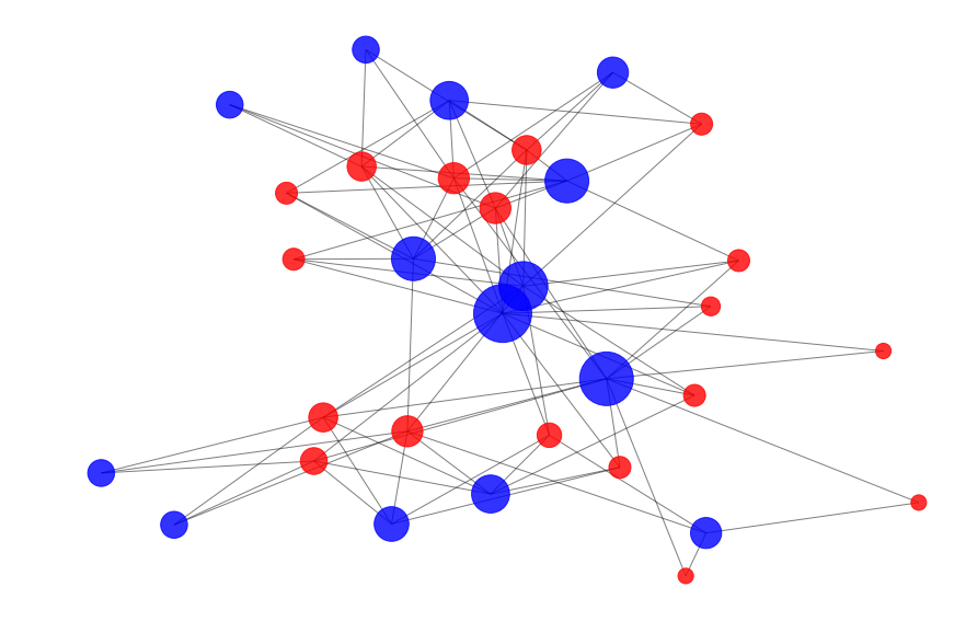
Let’s take a quick peek at this network. We’ll draw the women as smaller red nodes (with size relative to their degree centrality, or how many nodes they’re linked to) and the social events as larger blue nodes (again, with differential sizes based on how many nodes they’re linked to).
pos=nx.spring_layout(G) # positions for all nodes

# calculate degree centrality
womenDegree = nx.degree(G, women)
eventsDegree = nx.degree(G, events)

plt.figure(1,figsize=(15,10))
plt.axis('off')

# nodes
nx.draw_networkx_nodes(G,pos,
                       nodelist=women,
                       node_color='r',
                       node_size=[v * 100 for v in dict(womenDegree).values()],
                   alpha=0.8)
nx.draw_networkx_nodes(G,pos,
                       nodelist=events,
                       node_color='b',
                       node_size=[v * 200 for v in dict(eventsDegree).values()],
                   alpha=0.8)

# edges
nx.draw(G,pos,width=1.0,alpha=0.5)
<matplotlib.collections.LineCollection at 0x151c46a2b0>
Step 5: Examine one node type – women.
Let’s concentrate first the women nodes.
Basic Centrality Measures
Centrality measures are metrics that reflect “connectedness”. You can measure the sheer number of connected nodes (degree centrality), or use more sophisticated methods that count connectedness to well-connected nodes as more important than connectedness to weakly connected nodes.
We certainly see that some women have greater connectedness than others, because we made the node size for these women proportionally larger. Let’s check out their degree centrality, which we already calculated for plotting purposes.
We’ll make this easy to look at by doing the following:
- Create a data frame that we’ll populate with two columns
- Turn the object womenDegree into a dictionary (key-value pairs)
- Take that dict and turn it into the two columns of our data frame (one for keys, one for values)
- Order that data frame by degree.
womenDegreeDF = pd.DataFrame()
womenDegreeDF['woman'] = dict(womenDegree).keys()
womenDegreeDF['event_connections'] = dict(womenDegree).values()

womenDegreeDF.sort_values(by='event_connections', ascending = False)| woman | event_connections | |
|---|---|---|
| 0 | Evelyn Jefferson | 8 |
| 16 | Theresa Anderson | 8 |
| 4 | Nora Fayette | 8 |
| 7 | Laura Mandeville | 7 |
| 12 | Brenda Rogers | 7 |
| 17 | Sylvia Avondale | 7 |
| 3 | Katherina Rogers | 6 |
| 14 | Helen Lloyd | 5 |
| 6 | Myra Liddel | 4 |
| 5 | Ruth DeSand | 4 |
| 1 | Verne Sanderson | 4 |
| 10 | Charlotte McDowd | 4 |
| 11 | Frances Anderson | 4 |
| 2 | Eleanor Nye | 4 |
| 8 | Pearl Oglethorpe | 3 |
| 13 | Dorothy Murchison | 2 |
| 15 | Olivia Carleton | 2 |
| 9 | Flora Price | 2 |
It seems like Theresa Anderson, Evelyn Jefferson, Nora Fayette, Sylvia Avondale, Laura Mandeville, and Brenda Rogers are the social butterflies of the group.
Step 5: Projecting
Do our “social butterflies”, who frequent social events, have more acquaintanceships and interact with more women? Or are some of them “clique-ish” and always see the same people over and over? Let’s look at acquaintanceships!
We can do this by projecting our bipartite graph onto women nodes. That means collapsing the network to women only, constructing edges representing relationships between women which are mediated by both women being connected to the same event.
We’ll first check it out graphically and then numerically.
W = bipartite.projected_graph(G, women)
plt.figure(2,figsize=(15,10))
nx.draw_shell(W, with_labels = True)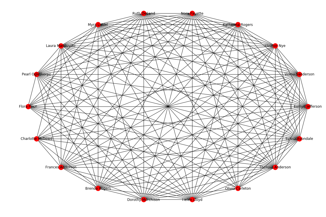
Wow, that’s lovely, but doesn’t tell us much. Let’s crunch the numbers! For variety, we’ll display a table using slightly different syntax than we used previously.
womenAcquaintanceship = pd.DataFrame({'woman': [w for w in women], \
                                'acquaintance_count': [W.degree(w) for w in women]})
womenAcquaintanceship.sort_values(by='acquaintance_count', ascending = False)| acquaintance_count | woman | |
|---|---|---|
| 0 | 17 | Evelyn Jefferson |
| 5 | 17 | Ruth DeSand |
| 16 | 17 | Theresa Anderson |
| 14 | 17 | Helen Lloyd |
| 1 | 17 | Verne Sanderson |
| 17 | 17 | Sylvia Avondale |
| 4 | 17 | Nora Fayette |
| 6 | 16 | Myra Liddel |
| 8 | 16 | Pearl Oglethorpe |
| 13 | 16 | Dorothy Murchison |
| 3 | 16 | Katherina Rogers |
| 7 | 15 | Laura Mandeville |
| 11 | 15 | Frances Anderson |
| 12 | 15 | Brenda Rogers |
| 2 | 15 | Eleanor Nye |
| 15 | 12 | Olivia Carleton |
| 9 | 12 | Flora Price |
| 10 | 11 | Charlotte McDowd |
We have seven women who have socialized with every other woman in our data set: Theresa Anderson, Helen Lloyd, Evelyn Jefferson, Nora Fayette, Sylvia Avondale, Verne Sanderson, and Ruth DeSand.
Step 6: Combining data
What would it look like if we combined what we know about women and look both at their connection to events and to each other?
womenSocialActivity = womenDegreeDF.merge(womenAcquaintanceship)
womenSocialActivity.sort_values(by=['event_connections', 'acquaintance_count'], ascending = False)| woman | event_connections | acquaintance_count | |
|---|---|---|---|
| 0 | Evelyn Jefferson | 8 | 17 |
| 4 | Nora Fayette | 8 | 17 |
| 16 | Theresa Anderson | 8 | 17 |
| 17 | Sylvia Avondale | 7 | 17 |
| 7 | Laura Mandeville | 7 | 15 |
| 12 | Brenda Rogers | 7 | 15 |
| 3 | Katherina Rogers | 6 | 16 |
| 14 | Helen Lloyd | 5 | 17 |
| 1 | Verne Sanderson | 4 | 17 |
| 5 | Ruth DeSand | 4 | 17 |
| 6 | Myra Liddel | 4 | 16 |
| 2 | Eleanor Nye | 4 | 15 |
| 11 | Frances Anderson | 4 | 15 |
| 10 | Charlotte McDowd | 4 | 11 |
| 8 | Pearl Oglethorpe | 3 | 16 |
| 13 | Dorothy Murchison | 2 | 16 |
| 9 | Flora Price | 2 | 12 |
| 15 | Olivia Carleton | 2 | 12 |
Step 7: Come up with preliminary insights
By looking at degree centrality and adjacency, we can tell that there are five women who have socialized both at the highest frequency (number of social events = 8) and with the greatest broadness (number of women they’ve co-attended with = 17):
- Theresa Anderson
- Nora Fayette
- Evelyn Jefferson
We also see women who have managed to rub elbows with every other woman in our data set, while not attending as many social events, most notably two women who have met everyone else while only attending four social events (which could be helpful info for the person who wants to meet a lot of people but not be socializing every night!):
- Verne Sanderson
- Ruth DeSand
In contrast to the high social efficiency of Verne and Ruth, we have Charlotte McDowd, who also attended four social events but only made connections with 11 acquaintances (the lowest number of anyone in the data set). Is Charlotte a bit more clique-ish than Verne and Ruth?
On the other end of the scale-of-sociability we see a couple of examples of women who have gone to the fewest social events (just two) and unsurprisingly have relatively low acquaintance counts:
- Flora Price
- Olivia Carleton
We can compare Flora and Olivia to the more socially efficient Dorothy Murchison, who also attended only two events, but managed to come out with 16 acquaintances, only missing one person.
My friend pick? Dorothy. She seems to both value her time as well as broad social connectedness with lots of different people. As a busy extravert, this appeals to me a lot!
Step 8: Ego Networks
Now that we have a few bellweather women to look more closely at, we can check out their personal networks. For example, let’s check out my new pal Dorothy’s network:
dorothy = nx.Graph(nx.ego_graph(G, 'Dorothy Murchison', radius = 2))
plt.figure(2,figsize=(15,10))
nx.d{% highlight python %}
{% raw %}(dorothy, with_labels = True)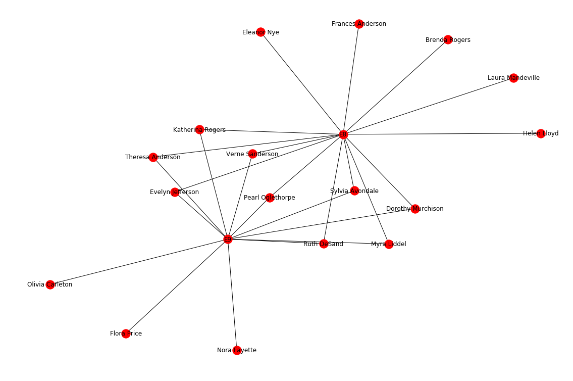
Dorothy attended two events, E8 and E9, which had great coverage between the two, when it comes to attendees. Let’s compare her to Charlotte McDowd, who attended twice as many events, but has a lower number of acquaintances:
charlotte = nx.Graph(nx.ego_graph(G, 'Charlotte McDowd', radius = 2))
plt.figure(3,figsize=(15,10))
nx.d{% highlight python %}
{% raw %}(charlotte, with_labels = True)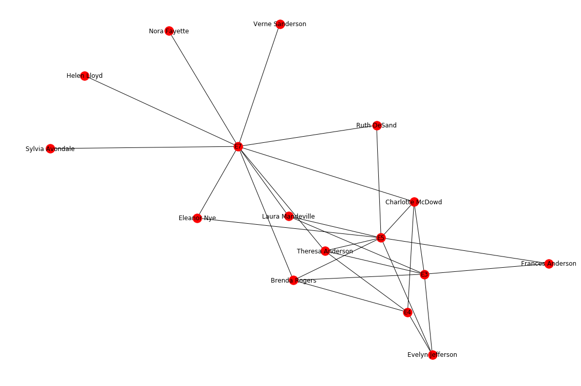
Charlotte’s ego network is much more tightly interconnected – she socializes at events which tend to have some of the same people. It looks like Brenda Rogers, Theresa Anderson, and Evelyn Jefferson are often found the same places as Charlotte.