R 4 Beginners

An exploration of data science as taught in R for Data Science by Hadley Wickham and Garrett Grolemund. This blog is meant to be a helpful addition to your own journey through the book. No prior programming experience necessary!

Chapter 1: Introduction and Installation

Who are we? Why are we here? What does it all mean?

Spoiler alert: I won’t answer that last question, at least not today. I won’t answer it primarily because I don’t know yet, but that’s the whole point, right? We’re learning. By the end of this series, maybe together we can get close to discovering what it’s all about. At least when it comes to data science with R. You’re on your own for the rest of it.

So who are we? Well, we’re probably all R newbies (I certainly am, and so are the folks this blog is intended to help). But there could be lots of reasons someone might be interested in R for data science, whether they need to supplement their data analysis arsenal with new tools, are looking to pivot into a new career, or are just curious. My goal for this series is to create a kind-of “study guide” to the R for Data Science curriculum.

Which brings me to the all-important Details. The book R for Data Science by Hadley Wickham and Garrett Grolemund, which is the focus of this series, is 100% FREE (how often can you say that anymore?) and can be found at https://r4ds.had.co.nz/. I’ll be hitting the high points in my blog posts, but I will not be copying it word-for-word because 1) that would be wrong and 2) I don’t need to, because the book is FREE. Go check it out if you want to follow along. There is a physical copy you can order online, but as the digital version can be updated much more readily than a physical book I’m sticking with the digital.

Ready to get started? Let’s do it!

The What, How, and Why: Not Necessarily in That Order

If you’re still here, you probably have some idea about why you might want to learn more about data science in general, and R in particular, but I’ll go into why I’m interested. When I first became interested in data science, I was a technician in a neuroscience research lab, and had been for almost 10 years; I worked with data all the time. For most of those years, I never once thought about data science, even though I was a scientist who often worked with data. Why? It really came down to the fact that I almost always worked with small data. By that, I mean that our experiments usually generated data that could be recorded relatively easily on a spreadsheet, manually cleaned up, copied and pasted into a statistics program, and the figures generated from there. However, while there might be some pros to this approach (you see the data at every step, it requires very minimal technical know-how), there are certainly cons as well. With all of that hands-on time comes many more opportunities for error, and as many of you may be aware, this manual process does not scale well at all. Luckily, even with small data sets, many of the same principles and processes that are generally used for big data can still apply. Have I convinced you? If not, that’s okay. As we go forward we’ll be practicing on mostly small data (even if it doesn’t always seem like it). Hopefully you’ll see that, even though it seems like a lot of work to put in to learn a different way to do a thing you already know how to do, the effort will save you time in the long run, with the added benefit of reproducibility and scalability.

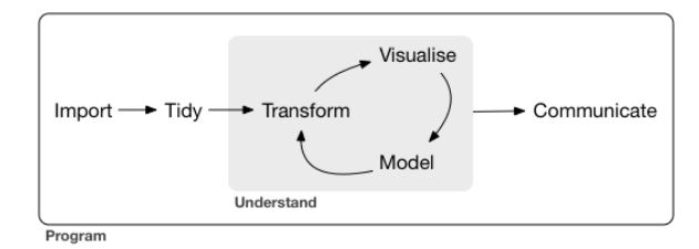
I pulled the image above from the introduction to R for Data Science (I’ll abbreviate this going forward as R4DS). It’s a simple schematic for the processes involved in data science. It’s a nice way to think about the tasks and tools involved. I’ll go through each step briefly:

• Import: We’ve got to get our data into the program we’re using before we can manipulate it. For those of us used to using statistical programs, I imagine that this step corresponds most closely with throwing all of our data into a spreadsheet in whatever form we get it; it may be messy, but at least it’s all in one place.
• Wrangle: This is the umbrella term for the process of tidying and transforming our data.
  • Tidy: You may also hear “data tidying” referred to as “data cleaning.” The idea is that before we can do anything else our data need to follow a consistent set of rules. For “tabular” or “rectangular” data, they are as follows:
    1. Each variable is one column
    2. Each observation is a row
    3. One piece of data per “cell” Making our data follow these rules early in the process will save us time and heartache later.
  • Transform: This is the step where we will “zoom in” on the data we actually want to work with. This might include a number of tasks, such as narrowing the data to just the subset we’re interested in (looking at a specific timeframe or zip code, for example), calculating new variables based on our newly tidy data (like converting a measure to different units or scale, or calculating a sale price from list price and discount percentage), and/or calculating summary statistics (mean, median, etc.). This is kind of like transferring data to a statistics program, where it has to be in a certain format and then it can run its calculations.
• Visualization: Once you have all of the nice tidy data that you want, one of the fun parts you can do is make an actual visual representation of your data. This can take a lot of forms: bar charts, line graphs, word clouds… there are tons of options! Visualization is key for creating scientific figures (this is where visualization feeds into communication), but they are also invaluable for understanding your data and guiding your future questions.
• Modeling: In this step, you can use computation to answer the questions that are raised by the previous steps. As R4DS explains, although visualization and modeling are both used to understand the data, modeling scales better than visualization; computers are generally cheaper than people, believe it or not, and it isn’t dependent on humans for interpretation.
• Communication: Once you’ve got an understanding of your data, you want to share what you’ve learned, right?

R4DS starts their instruction with data visualization. Why not start at the beginning? They claim that visualization is more fun and less frustrating than importing and wrangling data. I know when I think of my work with data that it is always cooler to see a result than to organize and calculate, so it isn’t surprising to me. Visualization is also a good way to start generating questions. But before we start anything, we need to do a few things: download R, download RStudio, and install a few packages. If you already have these installed, you can skip these steps (though take a look and make sure you have all of the packages we’ll be using).

Downloading and Installing R: A Simple Step-by-Step

A note: It is recommended that you download R and RStudio, especially if you plan to continue learning R in the future. However, if you really don’t want to download anything to your computer, or can’t for some reason, there is another option. RStudio.cloud is, as the name suggests, a cloud-based version of RStudio, so nothing needs to be installed, and it has a free version. Read the guide to get started if that’s your preference, and skip down to the “Installing the Tidyverse” section. If you want to download R and RStudio, read on!

1. Go to https://cloud.r-project.org/
2. Click on the link for the download you want, depending on whether you have a Mac or a PC that runs Windows.
3. If you have never installed R before, click the base link. If you have… you probably know better than I do what you should do. On Windows the link is right at the top of the page, but if you’re on a Mac you might have to scroll down a bit.
4. Download the version of R you want (when in doubt, go with the latest version- at the time of this publication it is version 4.0.3).
5. If you have Windows, you’ll be asked a bunch of questions about things like where you want the file to be located, the components to be installed, the startup options… just go with the defaults. Mac users won’t have to worry about it (you’ll just need to move the file from your Downloads folder into Applications).
6. Open up the file and check it out! If all is well, you should see something like this:

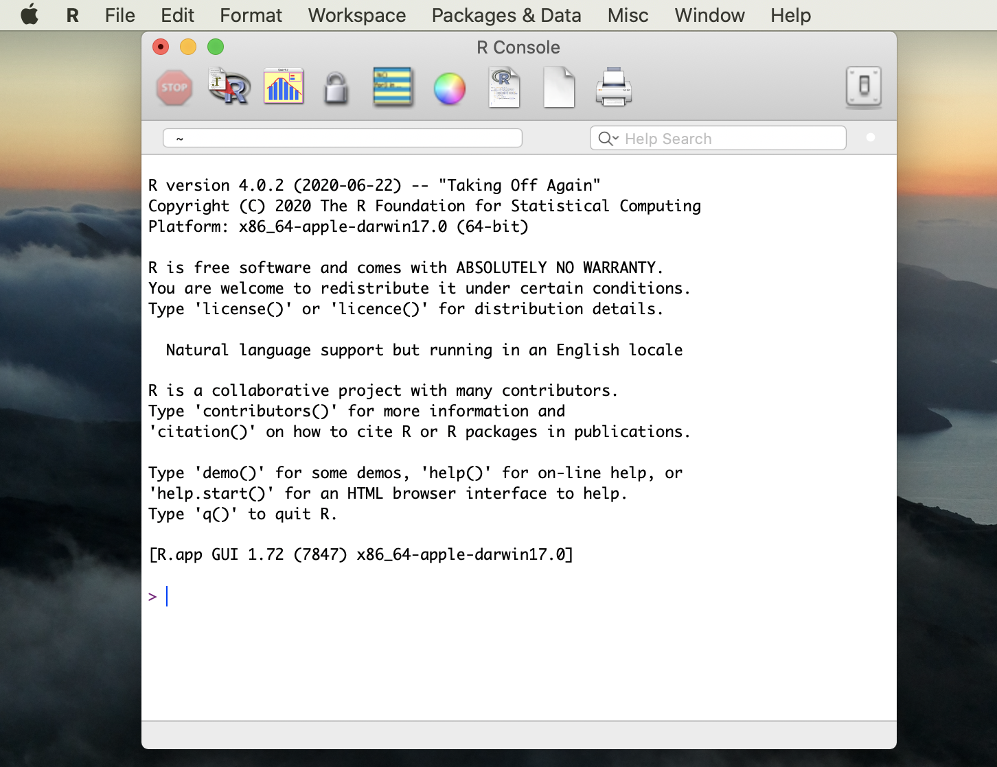
This is R’s graphical user interface, but don’t worry about it because we’re actually going to use another tool for coding in R: RStudio.

Downloading and Installing RStudio

RStudio is the integrated development environment (or IDE) that we’ll be using to write R code. While an IDE is not necessary for coding, it’s nice because you’ll generally have some built-in tools that will help you along the way. They contain a text editor, debugging tools, and other neat stuff.

1. Go to the RStudio website.
   • Note: Some of you, especially if you’ve worked with Python at all, might have Anaconda installed and have seen that you can install R and RStudio there. I don’t recommend it… mostly because I couldn’t get it to work. I’m going to stick to the instructions from now on.
2. Choose the version you want (might I suggest going with one of the FREE versions?). I went with the desktop version, but there’s a server version as well.
3. Hit that blue download button!
4. The website will recommend a download for your system. That’s the one you should probably just go with, but I would just double check that your system meets the requirements.
5. There might be some set-up to do.
   • If you’re using Windows:
   • You should see another Setup wizard. Hit “next.”
   • Like with R you’ll have to select destination and start menu folders for RStudio. Put it wherever, but I’d recommend putting it in the same location as R so that RStudio will be able to easily “find” R on your machine. If you just go with the defaults you should be good.
6. Once RStudio is finished installing, find it and open it- you’ll need it to install some packages.

Installing Tidyverse and Other Fun stuff

The R installation we’ve just downloaded does not contain all of the functionality we will use as we work through R4DS. The tidyverse is actually a group of packages that all work together and, as R4DS describes it, share a “common philosophy” of working in R. It is easy to install with our first line of code! Type the following in RStudio:

install.packages("tidyverse")

Be sure to include the quotation marks around “tidyverse”, they’re important! The installation may take a bit, so be patient. You will know it is finished when you see the file path and the blue “>”. Also, just a note, you might get a warning message about RTools being required to R packages… I figure that’s something we can go back and install if we need it later, so let’s not worry about it for now.

Next we need to load the tidyverse with another simple line of code:

library(tidyverse)

We will need to do this step every time we want to use the tidyverse (and we’ll be using it a lot!). Also, you may have noticed that there aren’t any quotation marks around tidyverse this time, because they aren’t necessary for this function (you actually can use quotation marks here if you want and it won’t give you an error… just in case you see it that way somewhere else).

That’s it, we’re all ready to get started! Next we’ll go through some of the basics of writing code.