
Null Hypothesis Statistical Testing (NHST)
Null Hypothesis Significance Testing (NHST) is a common statistical test to see if your research findings are statistically interesting. Its usefulness is sometimes challenged, particularly because NHST relies on p values, which are sporadically under fire from statisticians. The important thing to remember is not the latest p-value-related salvo in the statistical press, but rather that NHST is often best used alongside other measures that strengthen your claims, like effect size.
So what is null hypothesis statistical testing?
NHST is the statistical comparison of two means:
- an expected mean (like an IQ mean of 100) and observed mean (like mean IQ of children exposed to industrial pesticides in utero)
- group 1 and group 2, like the mean number of headaches in a placebo group and drug group
- the same group with two conditions (like mean face recognition accuracy before and after playing a violent video game)
As we know, any time you measure the mean of a sample, that mean could be larger or smaller than what you’re comparing it to just because of random chance. Or, the mean could be different because there’s a true difference between the two things you’re comparing. NHST helps us decide which possibility seems to be most supported by the evidence.
For example, let’s say I suspect that CHOP tends to have short employees more often than tall employees, because short people have a gene (CHOP1) that causes both shortness and an affinity for healthcare employment. Since men and women have height differences, we’ll concentrate our focus only on CHOP’s women employees, in order to simplify our investigation. I suspect their average height is lower than the average height for women generally.
One of these suspicions is empirically testable with NHST – does CHOP indeed have women employees that tend to be shorter than women generally? It is important to remember that null hypothesis testing cannot provide evidence to back up a claim of what caused a difference, but only evidence to back up the assertion that there is a difference. We can consider ourselves to have two hypotheses: a statistical hypothesis (we’ll find that CHOP-employed women are shorter than women generally), and a scientific or explanatory hypothesis (CHOP has shorter women because there’s a short-and-likes-healthcare gene that attracts short women to work at CHOP). Null hypothesis testing relates only to the statistical hypothesis.
I want to check my claim that CHOP’s female workforce really is different than women generally as far as height. I take a sample of 20 women employed at CHOP and discover that while the average height for women in the USA is 163.2 cm, the average height of our 20 female employees is 160.5 cm. The standard deviation of the sample is 10 cm. Now, the fact that the average height is lower than expected could just be random chance. After all, 20 is a small sample size, and I could have had weird luck and randomly picked 20 of the shorter women at CHOP.
Null hypothesis testing is like criminal prosecution. In criminal prosecution, the jury assumes that the defendant is innocent until proven guilty beyond a reasonable doubt. In our case, we assume that there’s no real difference happening, no real disparity between the height of women at CHOP and women generally, until evidence strongly indicates the contrary. Assuming “innocence” here is our null hypothesis.
The null hypothesis (H0) is always “nothing new or different is happening here, the means are the same.” In our case, the null hypothesis is that CHOP women actually have the same height, on average, as women generally. Sure, we might pick an unusually short or tall sample of CHOP women by happenstance, but the collection of all CHOP women is no different in height than women generally.
The “alternative hypothesis” (Ha) is that there really is a group difference, that the means are different. Your alternative hypothesis could be that the mean of the group you’re studying (CHOP-employed women, in our case) is larger than, smaller than, or different from (you don’t know which direction) the other mean. This “other mean” could be a different group you’re studying, or an expected mean, which in our case is the mean height of American women, which we believe is 163.2 cm. In our case, the alternative hypothesis is that the mean of women employed at CHOP is less than 163.2 cm.
The data we observed, the sample of 20 CHOP women with an average height of 160.5 and standard deviation of 10 cm, could conceivably occur under either hypothesis. So, did we just happen to get an unusually short group of 20 women from an otherwise totally average population? Or did we get a measurement that points to a real difference in the height of women at CHOP?
This is where we have to define our version of “reasonable doubt”. We’ll measure the probability that our sample would occur under the null hypothesis, and make the call based on that. What level of probability do we choose? Typically, we say 5% or 0.05. If the sample we observed has less than a 5% probability of occurring under the null hypothesis, we say we can reject the null hypothesis. That’s our “reasonable doubt”. Keep in mind that we’re admitting that on average, given a lot of “innocent” data, we’re going to get “false positives” around 5% of the time – we’ll reject the null hypothesis when we shouldn’t. This is why statistical significance is evidence, not proof. To make a strong claim, we rely on multiple measurements carried out at different times by different people that all demonstrate similar evidence. This is why replication is so crucial in science.
If you want to see the math of hypothesis testing illustrated and described simply yet in detail, you should definitely check out the Khan Academy videos on hypothesis testing.
In our case, we can do a T test which considers our sample measurements in cm (156, 155.8, 159.5, 174.6, 147.3, 163, 172.5, 156.1, 164.7, 170.1, 170.6, 161, 166.6, 149.8, 163.5, 145.8, 156.7, 158.2, 153.3, 164.1) and considers the likelihood of this sample coming from all CHOP women having an average height of 163.2 cm (the same as women in general). In R, I can use t.test:
> t.test(sample_chop, mu=163.2, alternative = "less")

	One Sample t-test

data:  sample_chop
t = -1.5051, df = 19, p-value = 0.07437
alternative hypothesis: true mean is less than 163.2
95 percent confidence interval:
     -Inf 163.6078
sample estimates:
mean of x
   160.46
My p value is 0.07437, so there’s a 7.437% chance that this sample belongs under the null hypothesis. That’s bigger than 5%, so we can’t reject the null hypothesis. We have to assume that CHOP women are no different than women generally, where height is concerned. Sure, we have kind of a short sample, but we can’t reject the possibility that we just had a sample that tended to be a little short, by random luck.
Now, what if I had a much larger sample, say, 2000 women at CHOP, with the same mean and standard deviation?
Consider what’s weirder: rolling 3 ones in a row with a die, or rolling 30 ones in a row with a die. We instinctively know that an unexpected outcome with just a few elements can happen pretty easily, and while it might draw our attention, we don’t jump to conclusions. But when the repetition of the unusual outcome gets bigger, we start to wonder what’s up. The T test is the same way – it is sensitive to changes in sample size. In the case of our 2000 woman sample, this could be our T test output:
> t.test(big_sample_chop, mu=163.2, alternative = "less")

	One Sample t-test

data:  big_sample_chop
t = -12.5, df = 1999, p-value < 2.2e-16
alternative hypothesis: true mean is less than 163.2
95 percent confidence interval:
     -Inf 160.8122
sample estimates:
mean of x
 160.4502
In this case, our p-value is so low it can’t be accurately calculated by my computer. Definitely way, way less than 0.05. We would therefore reject the null hypothesis and assert that we have some evidence to support the fact that CHOP women are shorter, on average, than women in general.
Our observed height difference is statistically significant, but is it really important or interesting? Are we noticing something that, while real, isn’t a big difference? In our case, the difference in means is less than 3 cm, which is pretty small. When we compare the difference between our groups with the difference within our groups (the natural variation in height, described as the standard deviation of 10 cm), we see that the effect size of “works at CHOP” is dwarfed by the natural variance of heights in either sample.
Cohen’s d is a commonly used effect size, and we can calculate it very simply. We take our sample mean (to be precise, it’s 160.45), subtract our H0 mean (163.2), and divide that difference by the standard deviation (we assume it’s 10 cm across the board). The figure we end up with, -0.275, shows that it’s a small effect size in the negative direction. Cohen suggested that d=0.2 be considered a ‘small’ effect size, 0.5 a ‘medium’ effect size, and 0.8 a ‘large’ effect size, but effect size is somewhat subjective and depends on the domain. For a company manufacturing machine screws for the space station, an effect size of ± 0.275 might be huge, while a chemotherapeutic drug trial might consider even an effect size of ± 0.8 to be small.
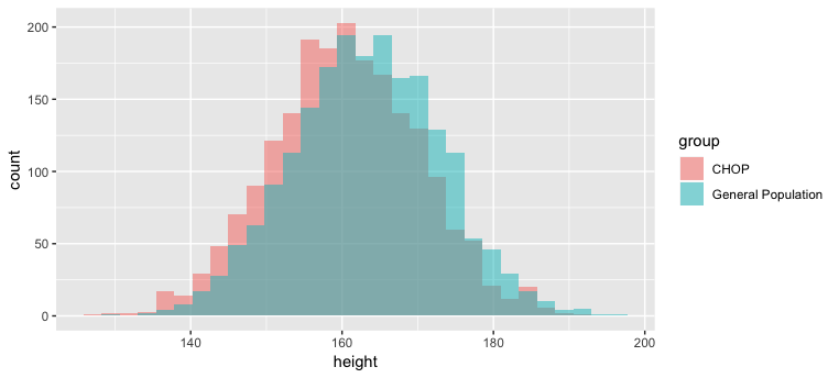
The use of effect size is a great way to contextualize findings. We had an extremely significant p value in our 2000-person sample, so we can be pretty confident in our assertion that CHOP women are clearly shorter than women generally (as long as we practiced good science in our sampling, etc.). But the difference? Not a big one, and probably not one anyone would ever notice or care about. When we plot our 2000 CHOP sample along with a 2000-woman sample from the general population, we see that there’s a difference, but not one that stands out a lot:
Want to learn more about hypothesis testing, including two-tailed tests (here I just covered a one-tailed test)? I recommend the charming and useful Handbook of Biological Statistics , particularly the section on hypothesis testing.